Table of Contents
Introduction
Now we begin the frequency divider (FD) design. We first examine the types of latches, which can be broadly classified into two categories: static and dynamic. After discussing the traits of these two latches, we then explain why dynamic latches are chosen over static latches. In the third section, we proceed with the actual design of our divide-by-120 FD in two different dynamic FFs. The design process will provide useful tips and highlight key design considerations throughout. Finally, we simulate the divide-by-120 FD in two FFs and cover its limitations. Then derive a new FF that consists of the advantage of prior FFs and conclude with the final divide-by-120 FD.
To keep things concise, we note “Divide-by-N FD” as “DivN” further on. {: .prompt-info }
1. Latch Styles
1.1. Static and Dynamic Latches
How to divide a signal
Now we begin the frequency divider design. How do we divide frequencies? For a given frequency, if we were to “hold” the signal and release it at the harmonic period of that frequency, we can divide the frequency. To do that, we need to make a circuit which operation runs on the input signal’s frequency. This behavior could be implemented by using latches, which could “hold” signals. Then, the concept could be advanced to Flip-Flops (FF), which are series of latches that could be operated by an “enable signal” By setting the enable signal to the input frequency of interest, we can derive a frequency divider.
Latch functionality
First, the static latches utilize back-to-back amplifying stages to store states. These circuits store the value by locking them in operating points, which inevitably demands the circuits to be powered on, frequently consuming power. Moreover, their topology naturally requires more transistors for its operation.
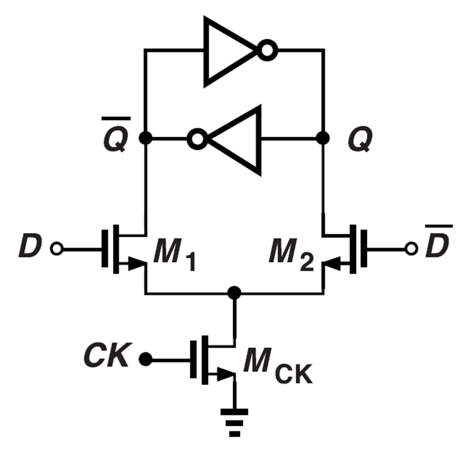
Figure 1. Static Latch with back-to-back Inverting Stages
Second, there are dynamic latches. These latches use their device capacitances to store value. They can be implemented with fewer transistors than static latches but may lose their states if the clock frequency is not sufficiently high.
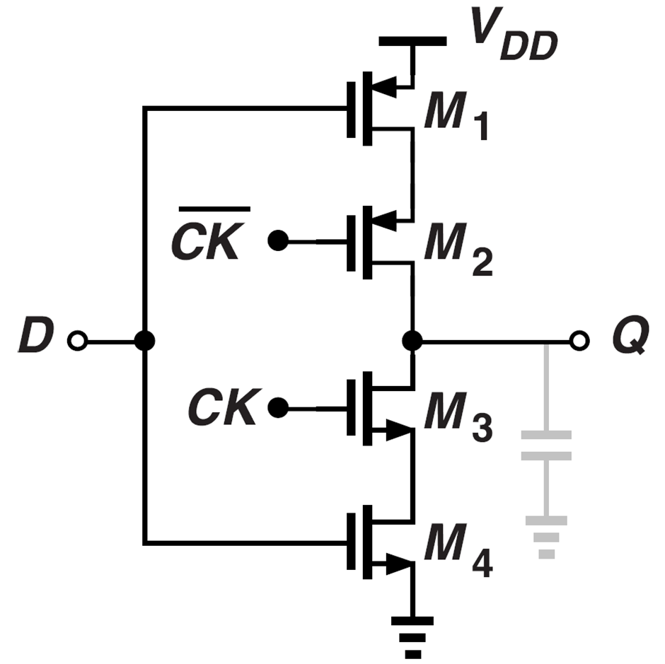
Figure 2. Dynamic Latch, "Clocked CMOS" ($ \small {\mathbf C^2 \mathbf {MOS}} $) Latch
Purpose of the Design
In this design, we target dynamic latches due to their advantages in low power consumption and to test how these dynamic latches behave in GHz topology.
2. Dynamic Latch
2.1. Proposed Latch
Among various types of dynamic latches noted in [2], fig.3 and fig.5 are the proposed topologies. For convenience, we will note them as “Comp SW FF” and “Ratioed TSPC FF” in short, respectively.
TIP: TSPC = True Single Phased Clock. {: .prompt-tip }
Comp SW FF
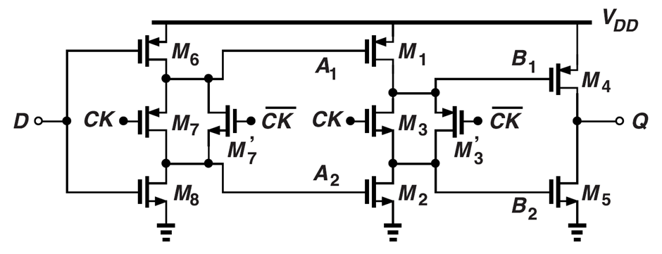

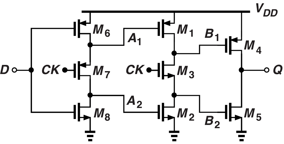

Comp SW FF can be implemented “unratioed” meaning there is no need for size considerations, and we could dive into the smallest dimensions, which is [W: 0.43um, L: 0.15um]. This design was originally a TSPC FF seen in fig.4, then later improved as fig.3 with complementary clocks to ensure faster operations in higher frequencies.
Ratioed TSPC FF
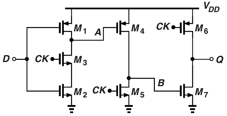

Ratioed TSPC FF could also be implemented “unratioed” and could be designed in the smallest sizes. Except for M_9, which should be two to three times wider for optimum speed.
While Ratioed TSPC FF seems like an intriguing option due to its fewer number of transistors. These Dividers have additional characteristics to highlight that cannot be spotted in textbook configurations. For further inspection, we move on to the actual designs to analyze its waveforms.
2.2. Design Simulation
Comp SW FF
Fig.6 is the actual implementation of Comp SW FF, fig.12 is the SPICE, and fig.13 shows the waveforms.
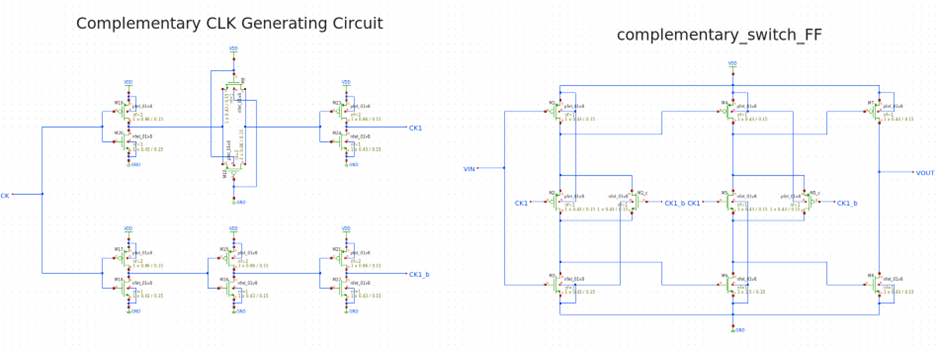
Figure 6. Schematic Representation of Comp SW FF
One thing to note is the complementary CLK generating circuit in fig.6. The development of such design develops from the concept in fig.7.
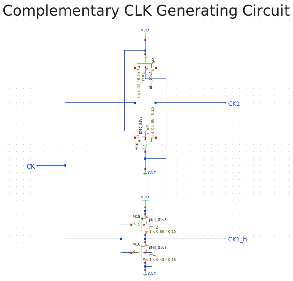
Figure 7. Complementary Clock Generating Circuit 1
The SPICE code for DC analysis is shown as fig.4, and its result is fig.5.
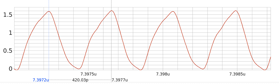
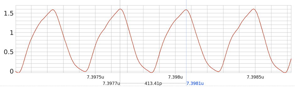
Figure 8. Complementary Clock Generating Circuit 2
Fig.8 shows the outcome where the PLL is built with Comp_sw_FF FD with fig.7 configurated complementary clock circuits. We can see the rising waveform is different between the periods of the signals. Therefore, fails in matching a 2.4GHz.
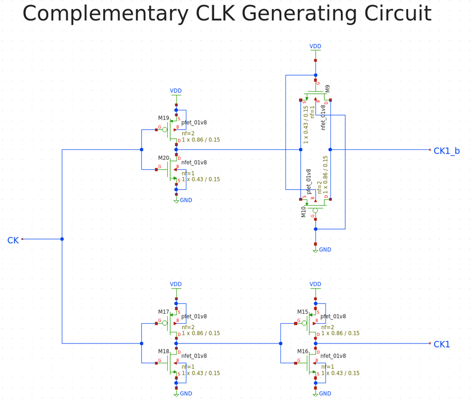
Figure 9. Complementary Clock Generating Circuit 2
We try to mitigate such traits with the addition of inverters to guard the VCO from the pass-gate. However, this design also provides subtle waveform mismatches in CK1_b and CK1 as shown in fig.9. This is also due to the pass-gate device.
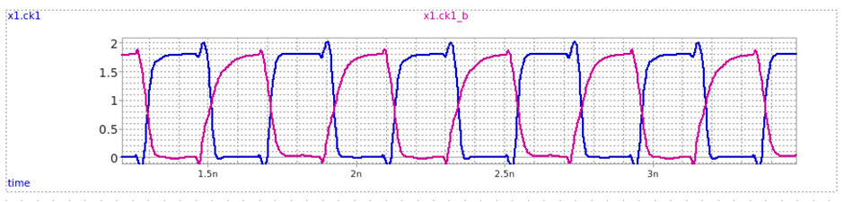
Figure 10. Waveform Mismatch
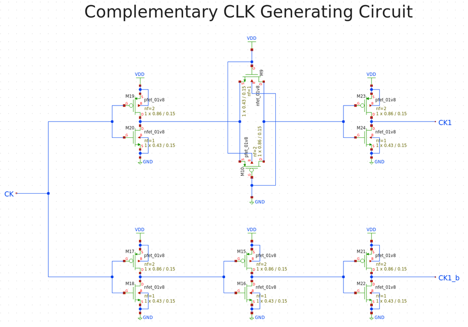
Figure 11. Complementary Clock Generating Circuit 3
In fig.11, we now guard both nodes of the pass-gate to suppress the parasitic capacitances. While this has disadvantages in delays, it has the best result in the simulation as in fig.13.
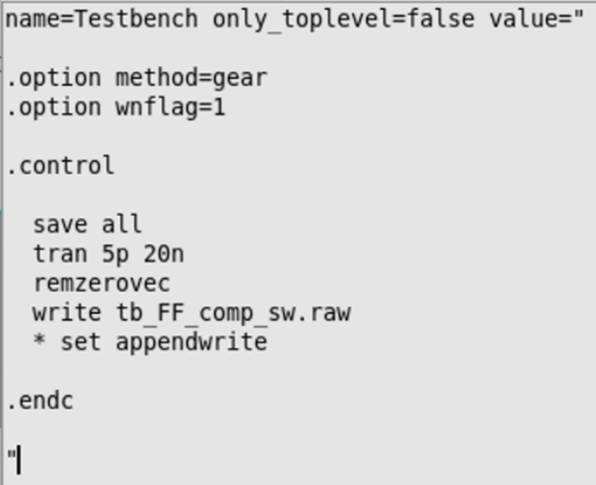
Figure 12. Comp SW FF SPICE
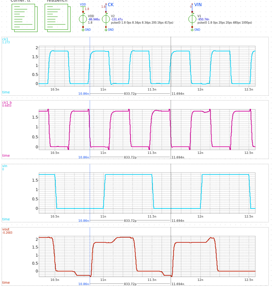
Figure 13. Comp SW FF Waveform
We can see that Comp SW FF is actually a Positive edge-triggered Flip-Flop with a single inverted output.
Ratioed TSPC FF
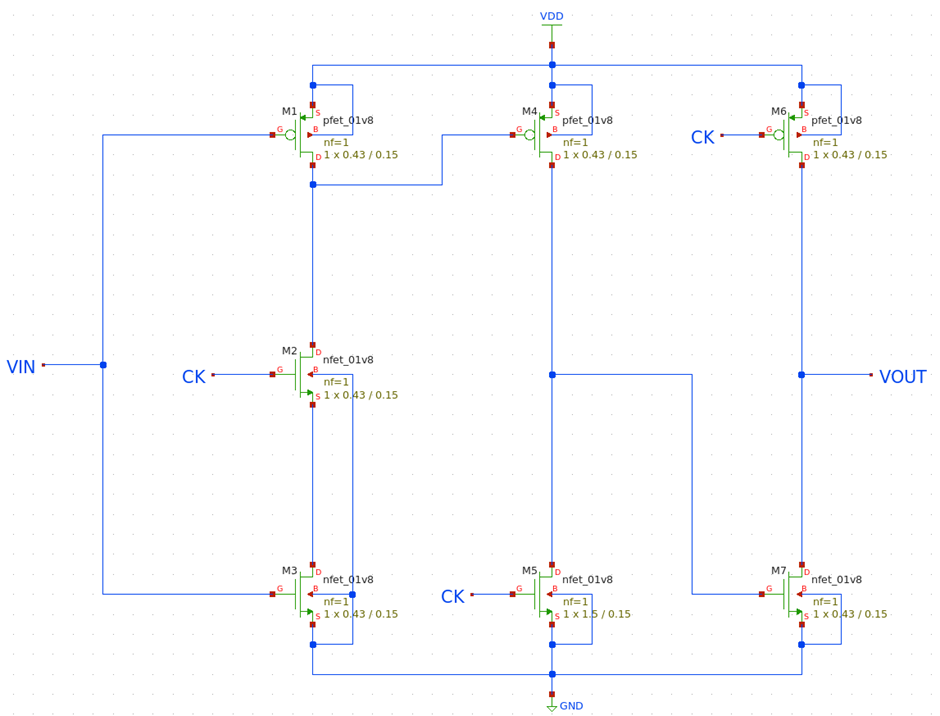
Figure 14. Schematic Representation of Ratioed TSPC FF
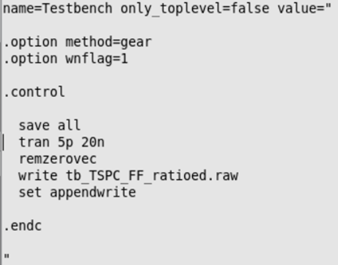
Figure 15. Ratioed TSPC FF SPICE
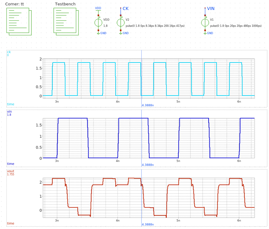
Figure 16. Ratioed TSPC FF Waveform
For the case of Ratioed TSPC FF, fig.14 is the actual implementation, fig.15 is the SPICE, and fig.16 shows the waveforms. By analyzing fig.16, we can understand for the case of Ratioed TSPC FF, it is a Negative edge-triggered Flip-Flop with a single inverted output.
One thing to note is that both TSPC FFs have inverting outputs, the reason for this could be that they all have three inverter stages. As for the Comp SW FF, [M1, M2, M2_c, M3], [M4, M5, M5_c, M6], [M7, M8] represent the three inverter stages, as shown in fig.6. Regarding the Ratioed TSPC FF, [M1, M2, M3], [M4, M5], [M6, M7] correspond to the three inverter stages, as shown in fig.14. This insight of treating FFs as a series of inverters is particularly beneficial when designing Div3 and Div5 components later in the post. We use a symbol such as fig.17, representing an FF with an inverting output.

Figure 17. Symbol of Inverting output FF
3. Proposed Dividers and Design Consideration
3.1. Divide-by-2 Design
3.1.1. Design Simulation
Comp SW FF
To make a Div2, we readily connect the “inverting” output to the input as fig.18 and fig.21. With the results illustrated in fig.20 and fig.23, the output is a signal with a period of 833ps, which is approximately of 2.4GHz.
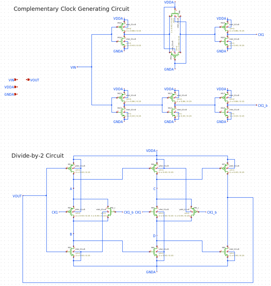
Figure 18. Schematic Representation of Comp SW FF Div2
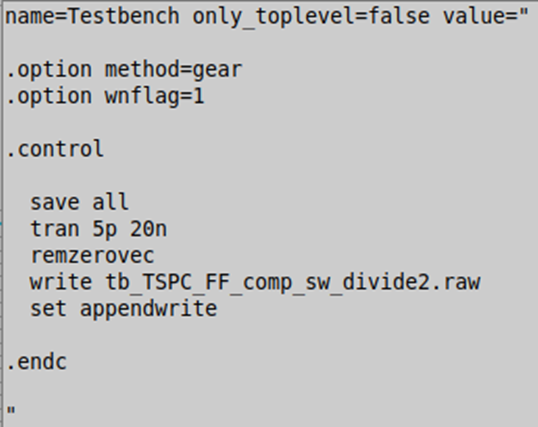
Figure 19. Comp SW FF Div2 SPICE
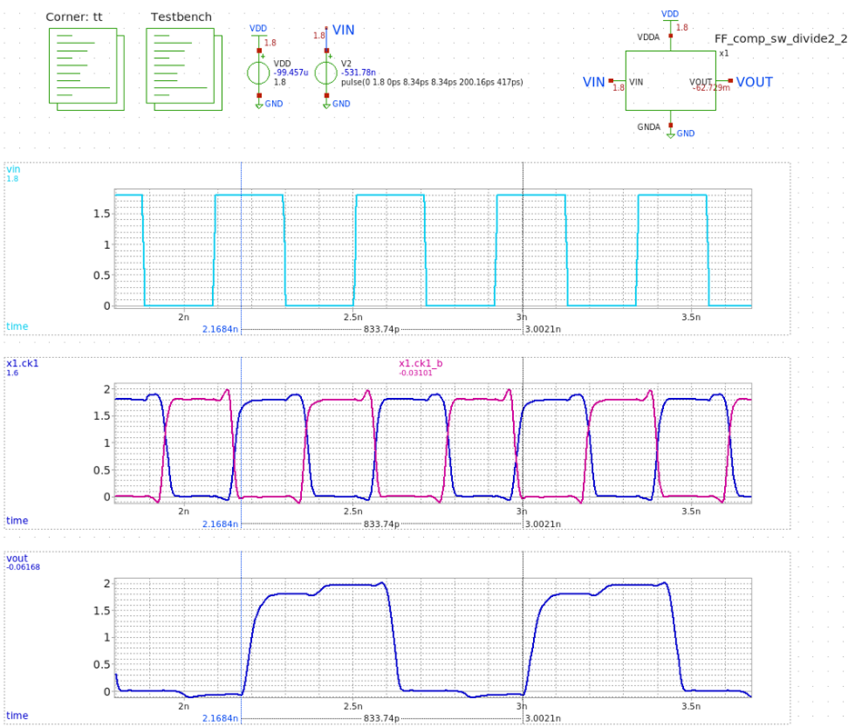
Figure 20. Comp SW FF Waveform
Ratioed TSPC FF
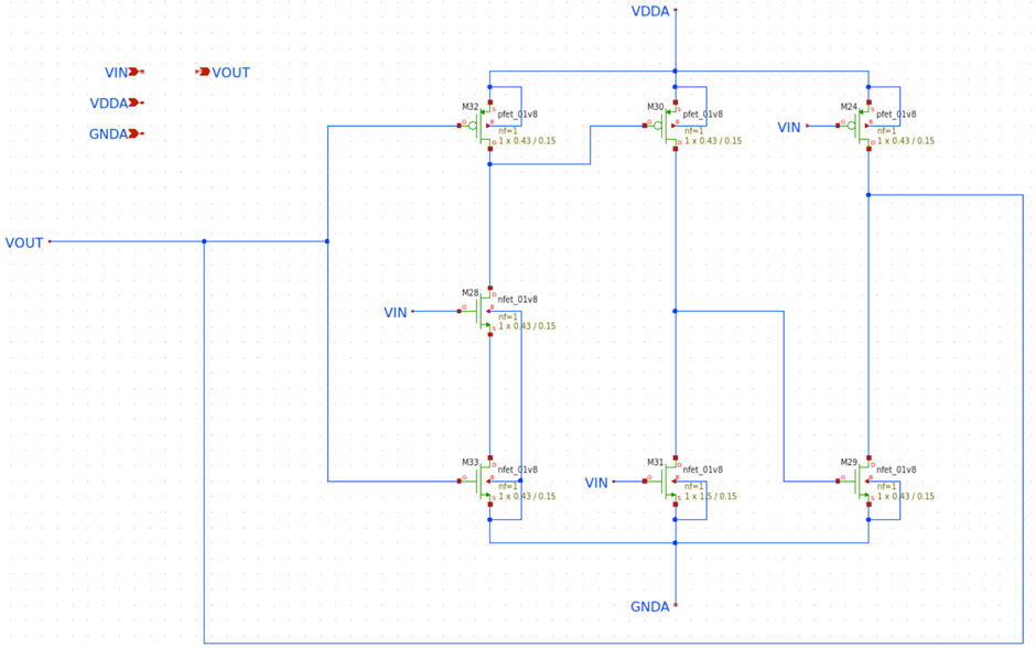
Figure 21. Schematic Representation of Ratioed TSPC FF Div2
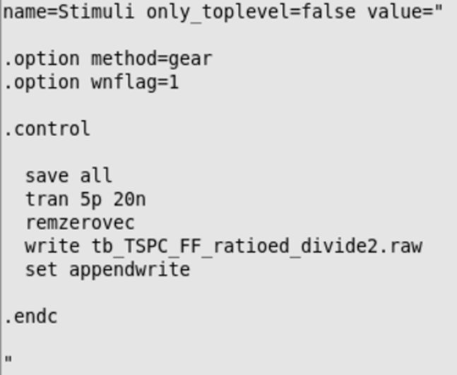
Figure 22. Ratioed TSPC FF Div2 SPICE
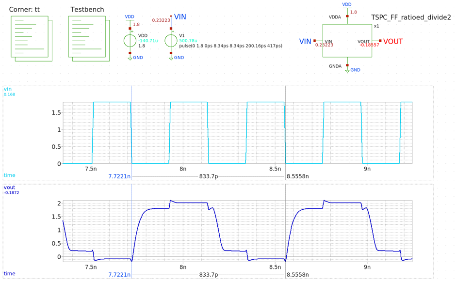
Figure 23. Ratioed TSPC FF Div2 Waveform
3.2. Divide-by-3 Design
3.2.1. Concept Development
Fig.24 is the proposed Div3 design from [2]. Unlike fig.17, this design features a non-inverting output.
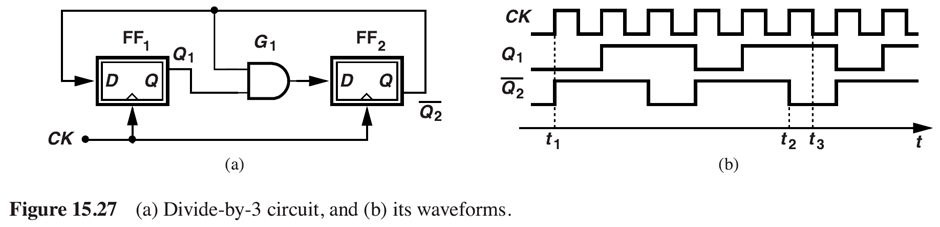
Figure 24. Div3 Concept
We change the FF to our configuration in then inspect how we can apply such an operation to our case. Also, note what we can do further to reduce the number of transistors.
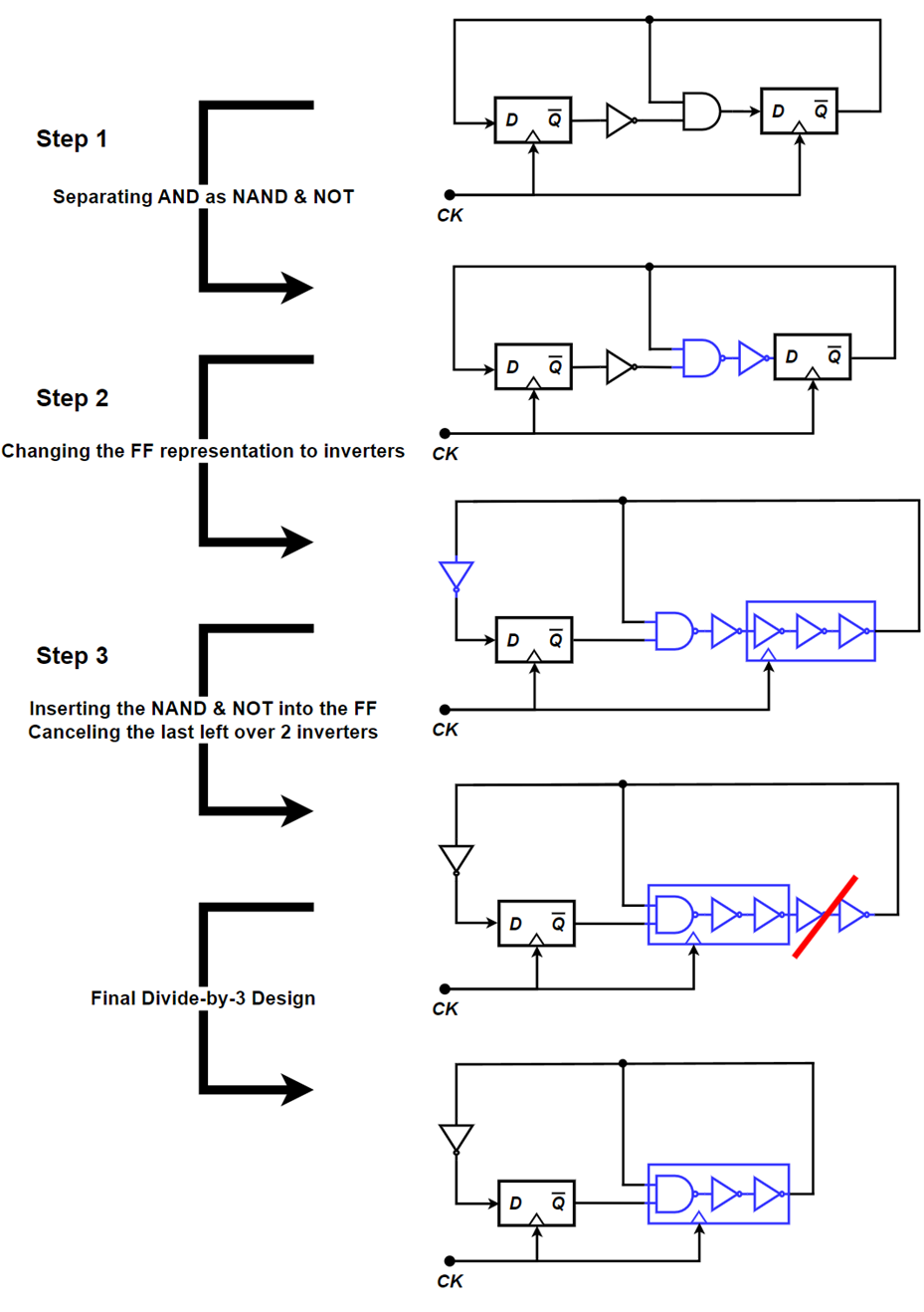
Figure 25. Process of applying the logic of fig.24 with fig.17, with improvements
Fig.25 shows the process of developing our own Div3
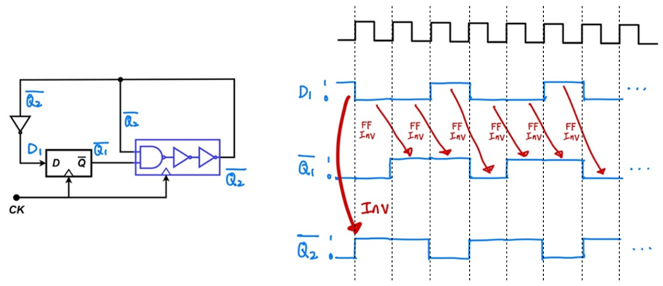
Figure 26. Hand-evaluation of the final Div3 circuit
Hand-Evaluation of Div3
Before the actual simulation of the FD, it is highly advised that the design be evaluated by hand. This is the best way for the designer to understand how logic works and if it matches our goal. Fig.26 presents an evaluation of the final Div3. However, it is recommended that each process step be manually evaluated individually, which I will leave as an exercise for the readers. A key starting point for those interested in attempting this would be setting the initial conditions for each node. To do this, select one node of interest and assign it an arbitrary value. This will allow the remaining node values to adjust according to the design’s logic configuration. If the design is correct, the circuit will produce a proper Div3 signal. Otherwise, it will converge to either a HIGH or LOW state.
Incorporation of a NAND Gate in the Flip-Flop (FF)
One thing to note in fig.25 is that we embedded a NAND into the FF. This is a legitimate approach because we agreed to develop the intuition that our TSPC FF is a series of three inverters. The key is to have three succeeding inverting stages grouped in the same clock. Even though we have a NAND instead of a NOT in fig.25, it still holds the purpose of carrying a state within its device capacitance.
Duty Cycle Considerations
Another thing to note is the duty cycle of this Div3 FD, which is shown in the waveforms in fig.24 and 26 as 66.6%. To prove that the phase and frequency distinguishing functionality is irrelevant to the duty cycle, we recall back the PFD design post. In that post, we explained that our PFD operates as a positive edge-detecting component. This means the window of interest spans from one rising edge of the signal to the next. Consequently, the duty cycle does not impact the functionality of this PLL’s topology, provided that the divided frequency adheres to the expected period.
3.2.2. Design Simulation
Comp SW FF
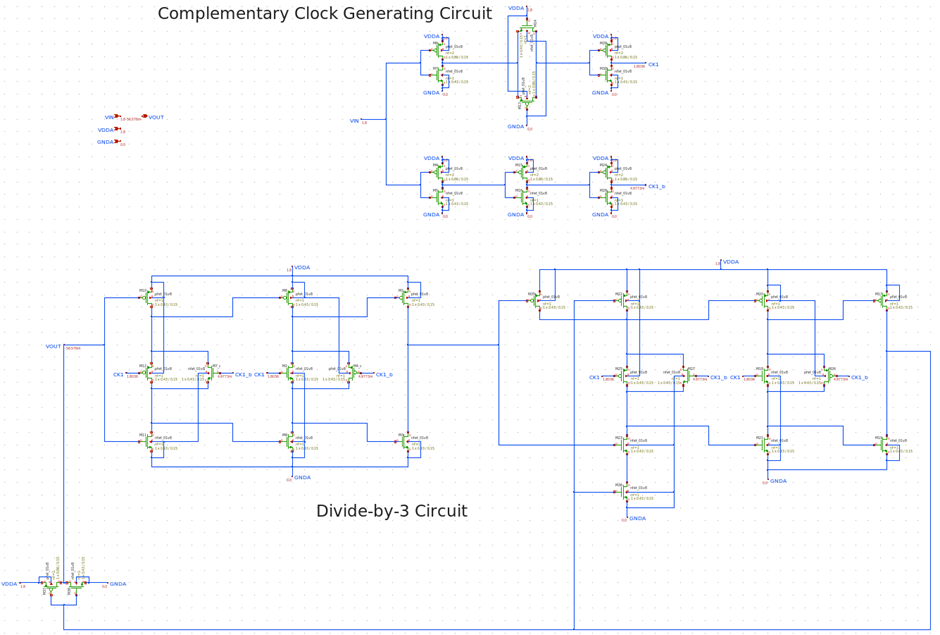
Figure 27. Schematic Representation of Comp SW FF Div3
Fig.27 is the transistor level Comp_sw_FF. Every NMOS and PMOS is sized [W: 0.43um, L: 0.15um] except for inverters and the pass-gates, which have PMOS as [W: 0.86um, L: 0.15um].
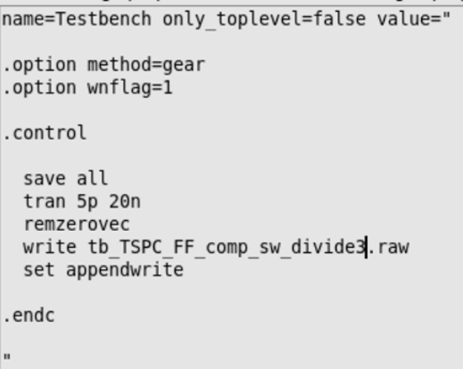
Figure 28. Comp SW FF Div3 SPICE
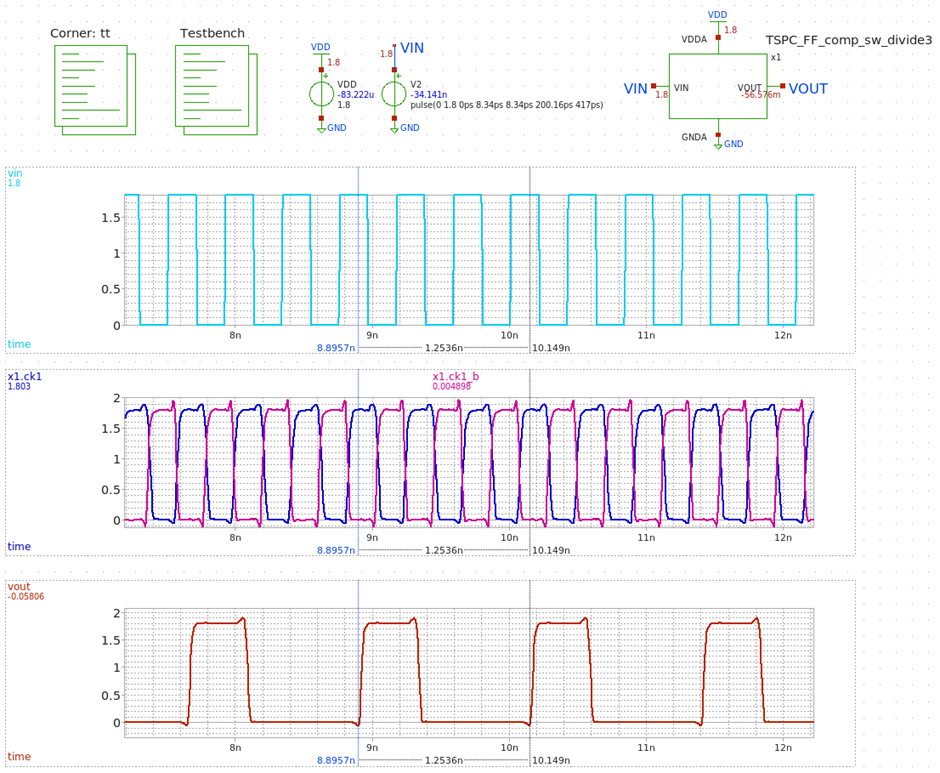
Figure 29. Comp SW FF Div3 Waveform
Ratioed TSPC FF
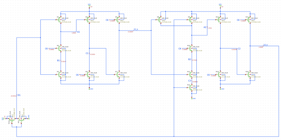
Figure 30. Schematic Representation of Ratioed TSPC FF Div3
Like the prior, fig.30 is the transistor level Ratioed TSPC FF. Every NMOS and PMOS is sized [W: 0.43um, L: 0.15um] except for inverters and the pass-gates, which have PMOS as [W: 0.86um, L: 0.15um].
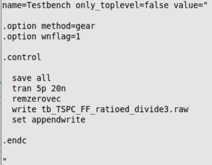
Figure 31. Ratioed TSPC FF Div3 SPICE
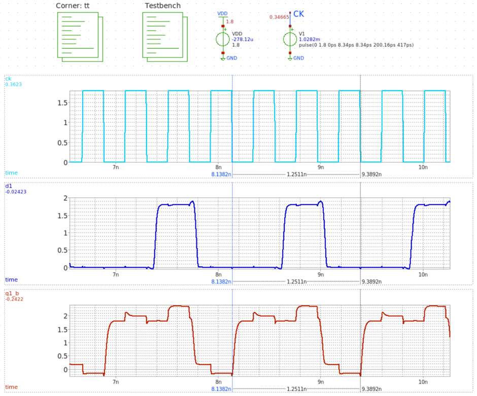
Figure 32. Ratioed TSPC FF Div3 Waveform
Same as before, fig.32 shows the waveforms of fig.30, which outputs a 1.2511ns signal, that is, of 2.4GHz.
3.3. Divide-by-5 Design
3.3.1. Concept Development
To make a Div5, we introduce the concept of a Dual Modulus Prescaler.
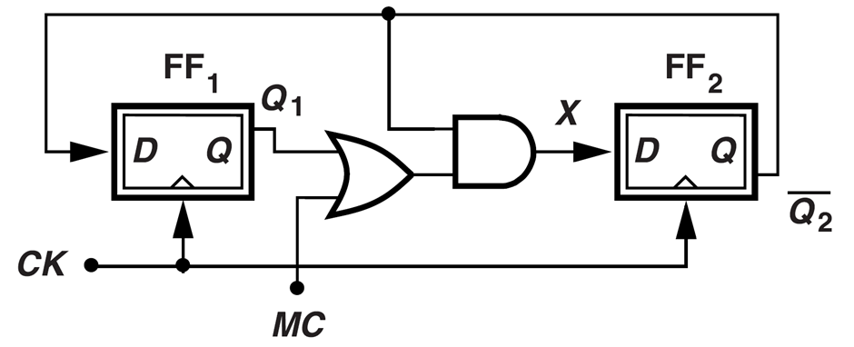

A dual modulus prescaler is a frequency divider that can switch between two division factors, likely N and N+1. By leveraging this characteristic, if N is 2, the prescaler can operate as a Div2 followed by a Div3. The summation of the doubled and tripled periods can be used to create a 1/5 frequency signal, which will have a duty cycle of 40%, as the doubled period accounts for that 40%.
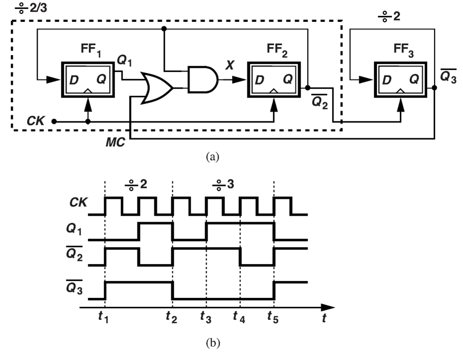

The dual modulus scaler, or the 2/3 (Div2,3) circuit, can be designed as fig.33. In [2], it adopts an OR gate to implement the “switch between two division factors” function. Then, it could be advanced into a Div5 as shown in fig.34.
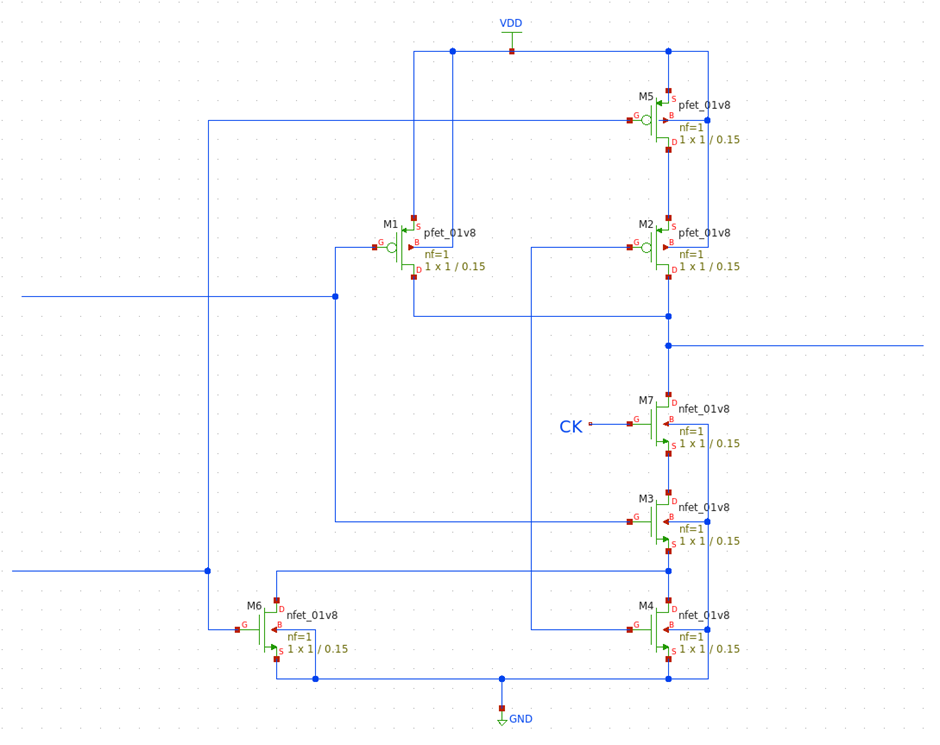
Figure 35. AND gate with OR input
Fig.35 shows how the AND & OR gates from fig.34 could be combined. If we manage to place the NOR component devices [M5, M2, M6, M4] near the rails, and NAND components [M1, M2, M3, M4] centered in the output node, it works as an “AND gate with OR input”
One interesting observation is that the AND with an OR input can be made with NAND with a NOR input. Combining two inverting-stage logic gates appears to nullify their respective NOT operations.
3.3.2. Design Simulation
Comp SW FF
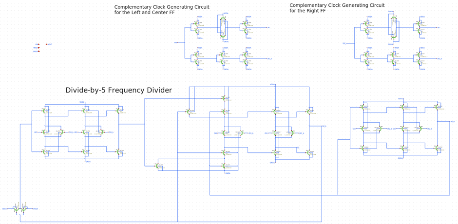
Figure 36. Schematic Representation of Comp SW FF Div5
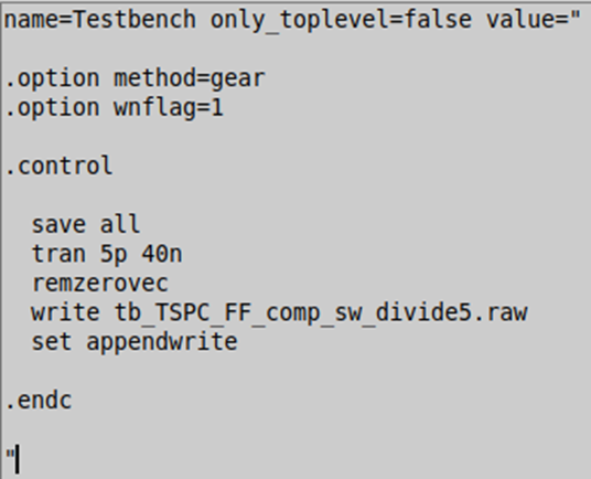
Figure 37. Comp SW FF Div5 SPICE
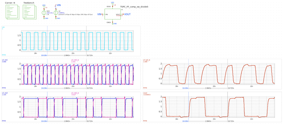
Figure 38. Comp SW FF Div5 Waveform
The vout signal in fig.38 shows a period of 2.0643ns, which is five times the period of a 2.4GHz signal.
Ratioed TSPC FF
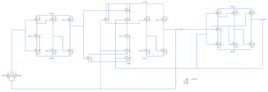
Figure 39. Schematic Representation of Ratioed TSPC FF Div5
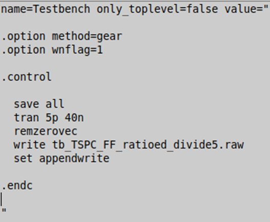
Figure 40. Ratioed TSPC FF Div5 SPICE
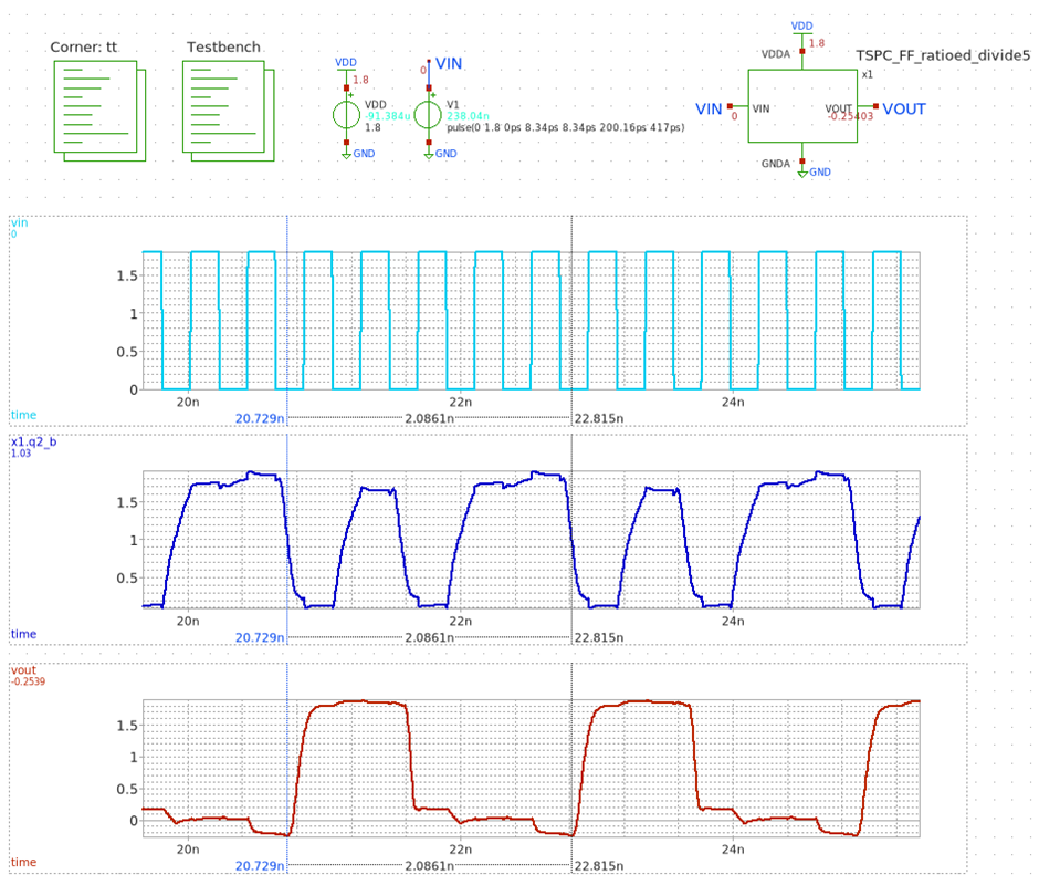
Figure 41. Ratioed TSPC FF Div5 Waveform
The vout signal in fig.22 shows a period of 2.0861ns, which is also five times the period of a 2.4GHz signal.
Now, with all three components that compose the Div120. We move on to its design implementation.
4. Divide-by-120 Design
4.1. Design Simulation
As we covered in the “PLL - Design parameters” post, 120 can be broken into . Meaning, Div120 can be built by connecting three Div2s, one Div3, and one Div5.
Comp SW FF

Figure 42. Comp SW FF Div120 Symbol Representation
For the Comp_sw_FF, the FD is implemented as fig.42, with the simulation setup like fig.44.
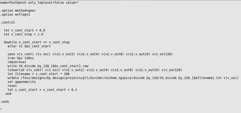
Figure 43. Comp SW FF Div120 SPICE
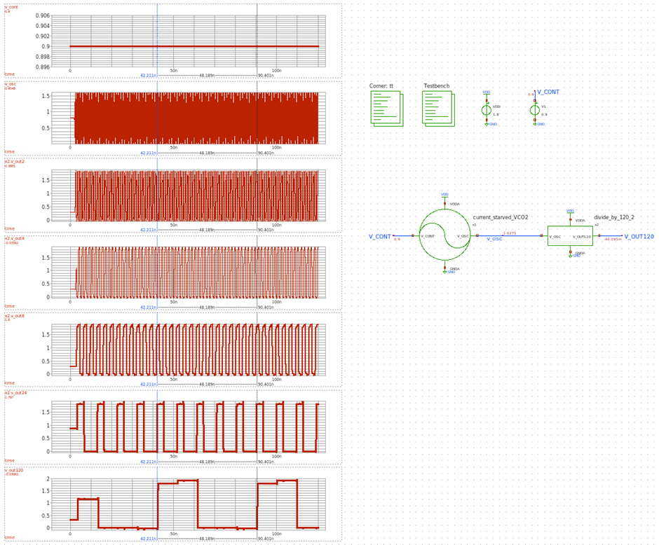
Figure 44. Comp SW FF Div120 Setup and Waveform
The SPICE is written as fig.43, where the code is written similarly to SPICE for evaluating the Kvco in the VCO post. The code measures up to 120ns which covers at least one period of the divide-by-120 (20MHz = 50ns). We write the code as such because, as we briefly mentioned in the last part of the VCO post, the capacitance from the FD influences the VCO, degrading its operation speed. So, we need to change the aspect ratio of the MOSFETs in the ringed oscillator so that it meets our frequency of interest, 2.4GHz.
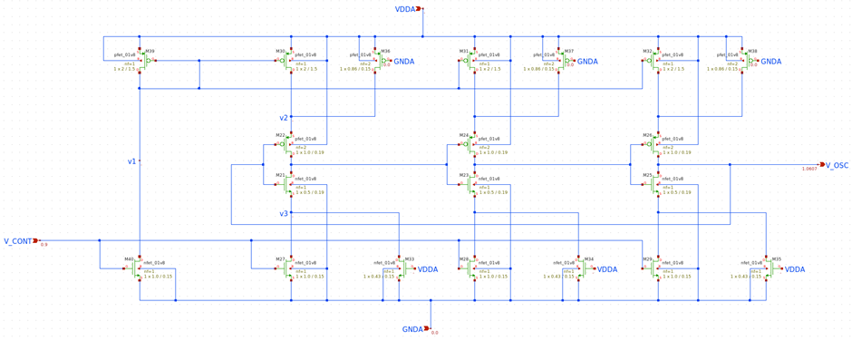
Figure 45. Revised VCO Schematic of Comp SW FF Div120
After changing the size from [W_p: 0.86um, L_p: 0.27um, W_n: 0.43um, L_n: 0.27um] to [W_p: 1.0um, L_p: 0.19um, W_n: 0.50um, L_n: 0.19um] as shown in fig.45. It creates a Kvco plot as fig.46.
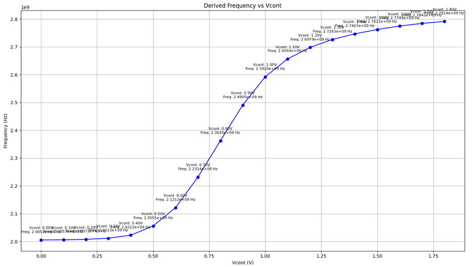
Figure 46. Kvco plot of the Revised VCO
With this revised VCO, the output frequency is for V_cont of 0.9V. When this goes through the FD, the period of the final signal is 48.177ns, as shown in fig.47.
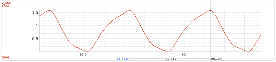
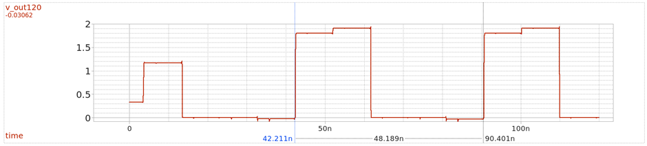
Figure 47. VCO output (Top), Div120 output (Bottom)
We can conclude that the FD successfully delivers divide-by-120 through the following calculation.
Ratioed TSPC FF

Figure 48. Ratioed FF Div120 Symbol Representation
For the Ratioed_FF, the FD is implemented as fig.48, and the simulation setup as fig.49. As explained above, the SPICE simulation is written similarly to serve the same purpose.
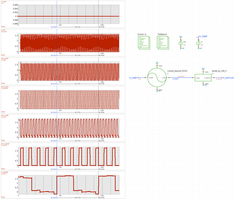
Figure 49. Ratioed TSPC FF Div120 Setup and Waveform
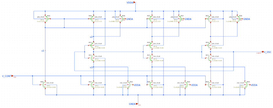
Figure 50. Revised VCO Schematic of Ratioed TSPC FF Div120
[W_p: 0.86um, L_p: 0.27um, W_n: 0.43um, L_n: 0.27um] to [W_p: 0.86um, L_p: 0.20um, W_n: 0.43um, L_n: 0.20um] as shown in fig.50. It creates a Kvco plot as fig.51.
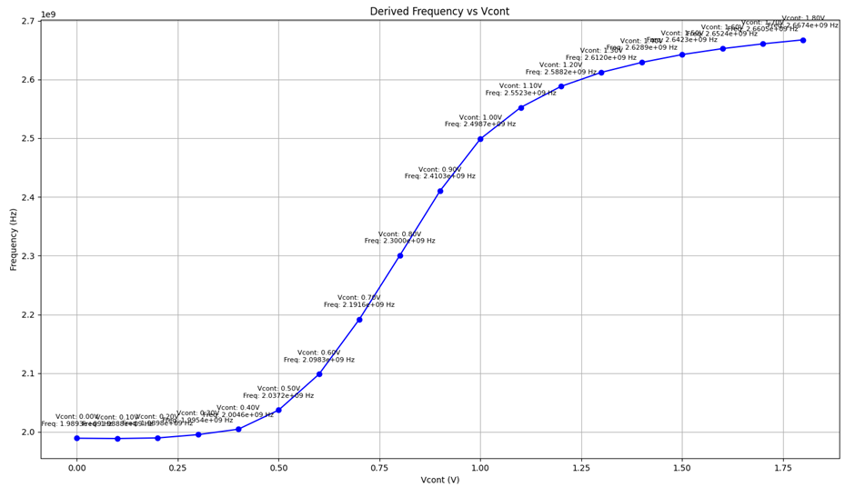
Figure 51. Kvco plot of the Revised VCO
With this revised VCO, the output frequency is for V_cont of 0.9V. When this goes through the FD, the period of the final signal is 49.755ns, as shown in fig.52.
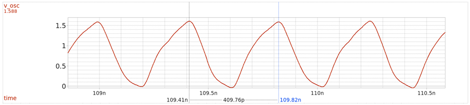
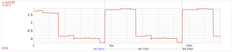
Figure 52. VCO output (Top), Div120 output (Bottom)
We can see that for the case of the Ratioed FF, the division ratio is , which is near 120. However, for those with a sharp eye, you can see that the VCO output signal in fig.52 is slightly distorted, as we first observed in fig.8.
4.2. Impact of the Divider
From fig. 7, 8, 9, 10, and 52, it was observed that parasitic capacitance poses a significant issue, as it distorts the VCO output signal when the divider is connected. This issue may be suppressed if the dimensions of the MOSFETs get smaller, but [W_n: 0.43um, L: 0.15um] is the lowest limit. Thus, we cannot derive a solution in this direction.
While the FD of Comp_sw_FF derives a solution from using inverters, it uses too many MOSFETs, even overwhelming the numbers used for FD design in divide-by-2. This leads to longer simulations because they vary proportionally to the number of devices, which is another inconvenience. Plus, the Comp_sw_FF topology introduces an additional disadvantage of delays from its complementary clock-generating stages.
4.3. Revised FF
Instead, an alternative can be drawn from the strengths of both approaches. We could choose the Ratioed FF for its merit in fewer devices while shielding the VCO & FD connection as much as possible using inverters as in comp_sw_FF.
The FDs directly connected to the VCO output node are the divide-by-2 and the divide-by-3. This is intuitively seen because the divide-by-2 is made by connecting the input and output of the FF. The divide-by-3 is related by having its input connected to that node.
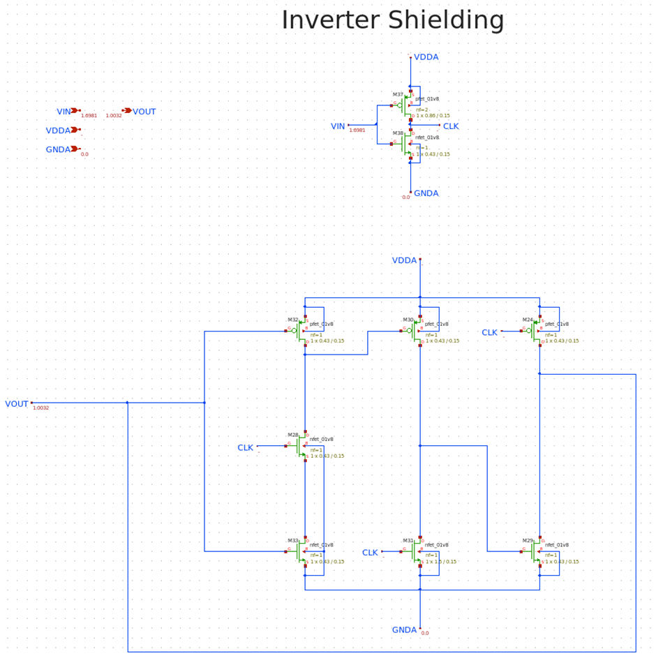
Figure 53. Ratioed TSPC Div2 with Inverter Shielding
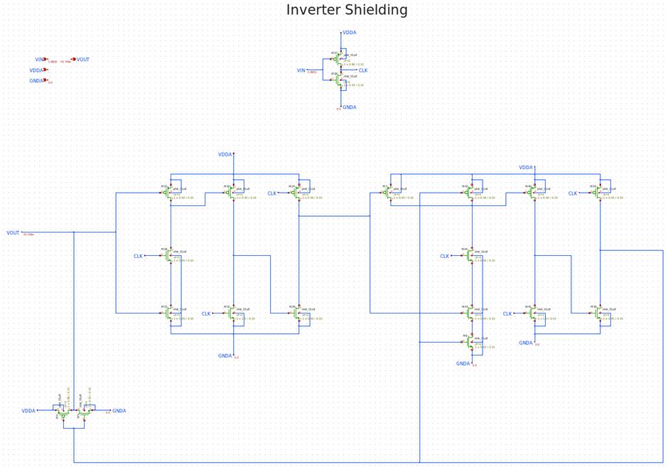
Figure 54. Ratioed TSPC Div3 with Inverter Shielding
Replacing the original divide-by-2 and divide-by-3 with the proposed FD design in Fig.53 and 54. We then examine how the actual operation under this solution behaves.
4.4. Final Evaluation
The simulation conditions are identical to the ones introduced in “4.1. Design Simulation.” Hence, we focus on the main points.
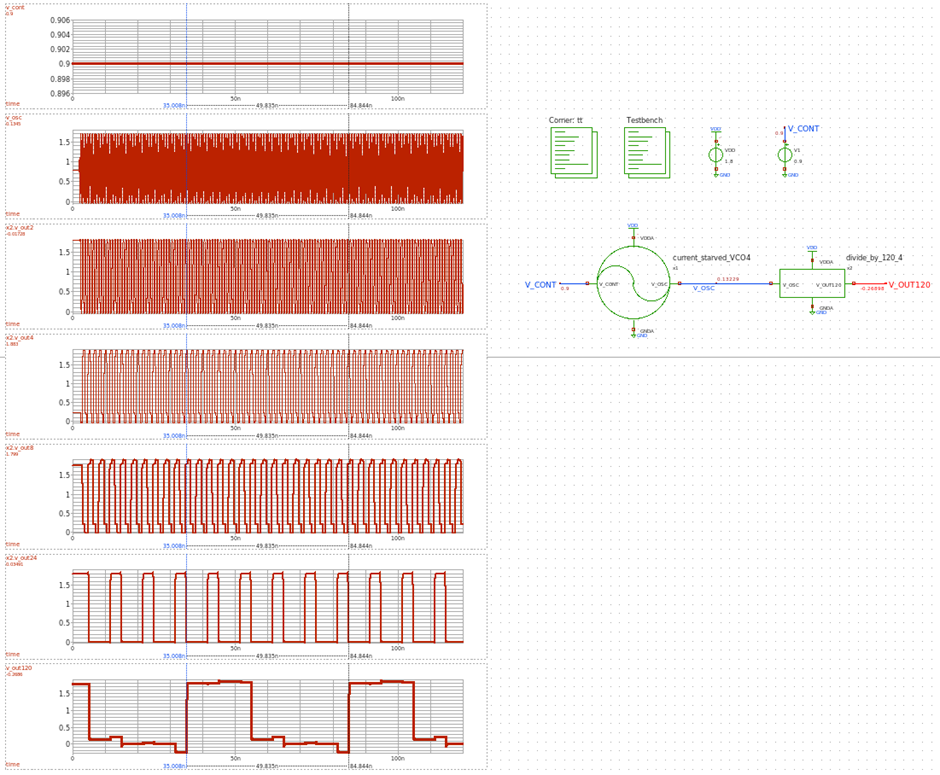
Figure 55. Final FF Div120 Setup and Waveform
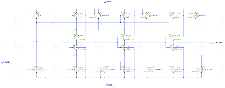
Figure 56. Revised VCO Schematic of the Final FF Div120
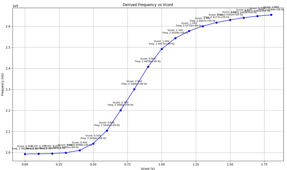
Figure 57. Kvco plot of the Revised VCO
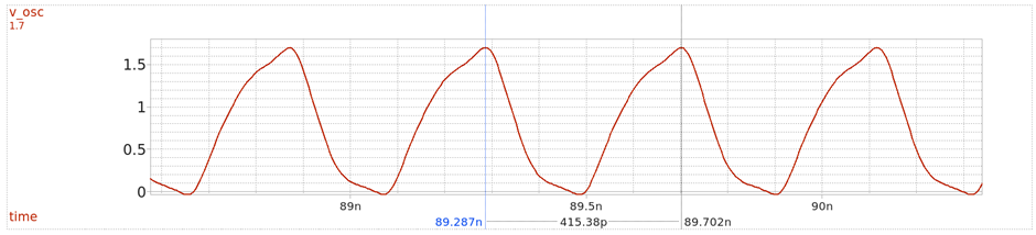
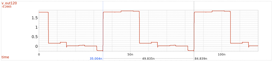
Figure 58. VCO output (Top), Div120 output (Bottom)
We see that with this VCO and FD, the VCO outputs for V_cont of 0.9V. Then to a divide-by-120 signal of 49.835ns, which leads to the divider factor of , promisingly matching up with our original concept.
Additionally, we can confirm that the VCO output signal (top image of fig.58) does not seem to be corrupted by the capacitances from the succeeding stages, resolving the issue from fig.54.
References
- [1] Design of Analog CMOS Integrated Circuits, 2nd Edition - Razavi
- [2] Design of CMOS Phase-Locked Loops: From Circuit Level to Architecture Level, 1st Edition - Razavi
Next post, the full topology of the PLL will be put under analysis.
Discussion
Comments
Share questions, corrections, or notes through GitHub.