Voltage Controlled Oscillator (VCO) Design Part 1
As its name implies, a voltage-controlled oscillator is an oscillator that can be controlled by some control voltage.
Starting off, we should begin by making the simplest current-starved oscillator.
Additionally, we will implement the smallest length and width in every transistor to check the maximum frequency of the VCO in the Skywater130-PDK environment. The NMOS and PMOS used in this design are “PMOS name” and “NMOS name.” By accessing its SPICE file, we can find out the minimum width is 430nm, and the length is 120nm.
Key Design Philosophy
Before starting off, one key point when creating designs is this excellent quote from Prof. Hajimiri from Caltech:
- Know your topologies.
- Then consider the aspect ratios (Width & Length).
It is okay to perform some aspect ratio checks while validating step 1. However, if you ignore this process and jump into design without fully understanding the knobs you are controlling, you will most likely end up in an endless maze, wasting precious time.
Initial VCO Design
We begin with the simplest design, shown in Figure 1, and Figure 2 explicitly demonstrates the functionality of the transistors.
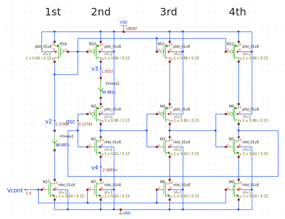
Figure 1 - Simplest VCO Topology
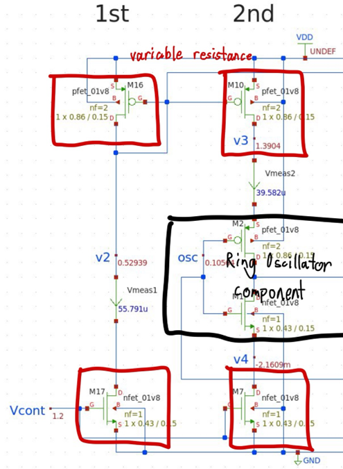
Figure 2 - VCO Functionality
The SPICE code for this design is as follows:
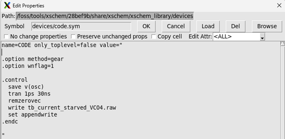
Our control voltage (V_CONT) is ambiguously set to 0.9V. This configuration saves the value of v(osc) in a .raw file. Viewing the waveform, it looks like this:
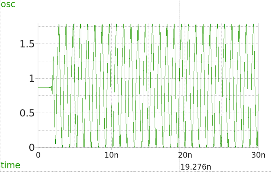
Figure 3 - Output Signal
From the transient response, we can directly measure the period. At our first attempt, the frequency is measured as 1.02 GHz. This is a promising result because now we may now be able to configure it to our target frequency of 2.4GHz.
Measuring Kvco
Why Measure Kvco?
To better understand the behavior of this VCO, we first measure the Kvco, as it provides essential insights before diving deeper into the design.
To measure Kvco:
- Sweep V_CONT: From 0V to 1.8V in 0.1V steps.
- SPICE Code: The SPICE code for this sweep is as follows:
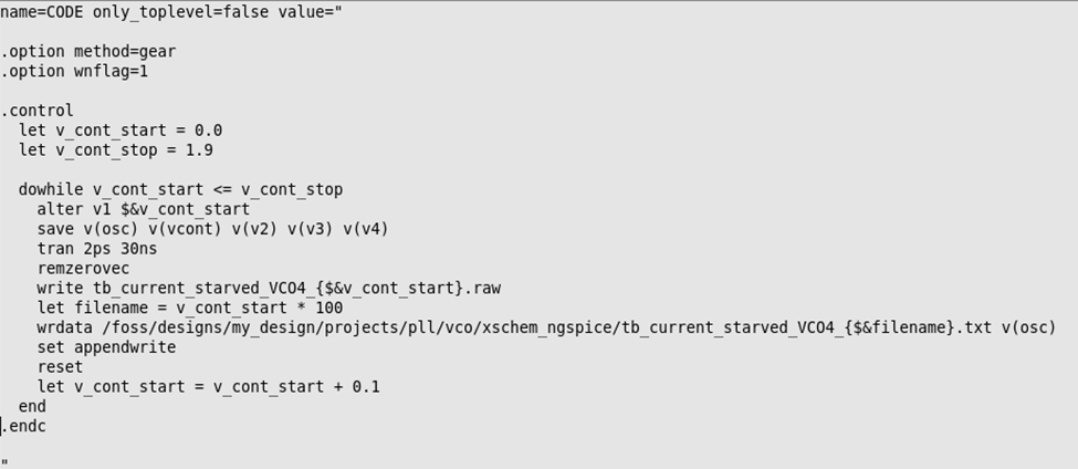
Note: After simulation,
.txtfiles will be generated. Convert these files to.csvfor easier examination using Python.
Automating Kvco Calculation
Manually measuring frequency from 19 raw files is tedious. To streamline this, I developed two Python scripts:
- convert_txt_csv.py: Converts
.txtfiles to.csv. - find_frequency.py: Finds frequency using the
find_peakslibrary in SciPy.
Python Code Details
- find_frequency.py: This script uses
find_peaksfor peak detection. Alternative methods, such as threshold crossing and FFT, were tested, butfind_peaksprovided the best results. - Offset Error: Note that the code introduces a 1% offset error compared to hand-measured frequencies. For quick Kvco measurements, this is acceptable, but final measurements should be done manually.
Kvco Results and Observations
The Kvco derivation process is as follows:
- Run SPICE Simulation.
- Run convert_txt_csv.py.
- Run find_frequency.py.
The output result is shown below:
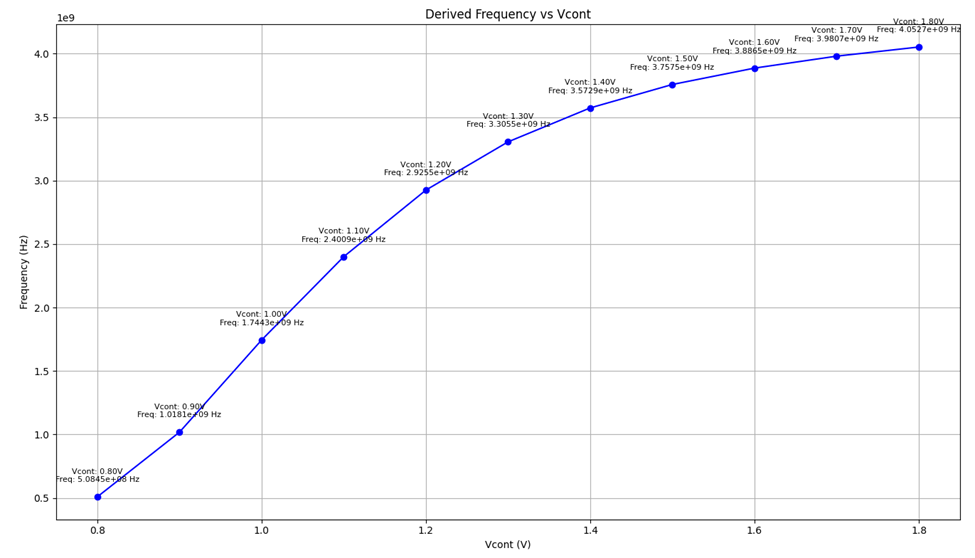
Figure 4 - Simplest VCO Kvco
Key Observations
- The Kvco is non-linear, which is undesirable.
- The VCO is inactive below certain voltage.
This is due to the current mirroring approach in this topology. When the PMOS and NMOS transistors in the first branch are in cutoff, no current is available to mirror.
Figure 5 demonstrates this behavior:
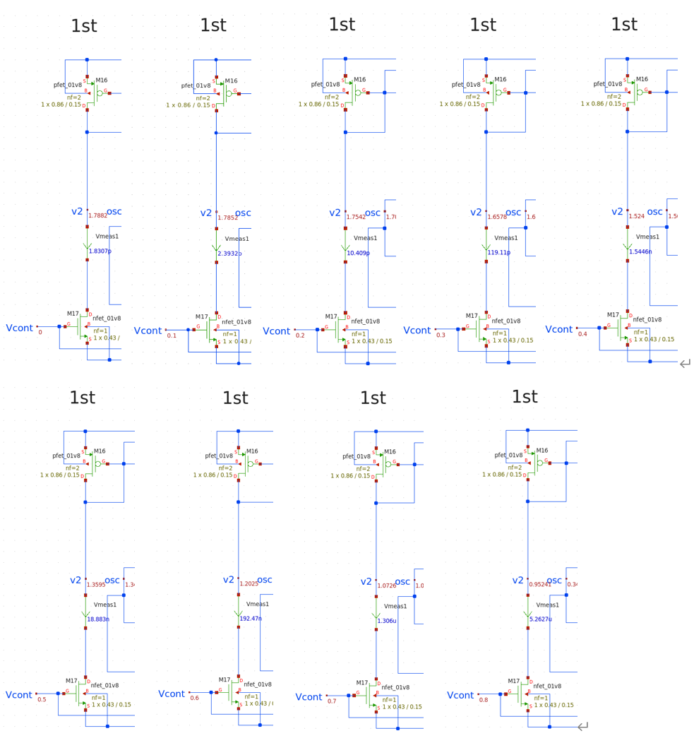
Figure 5 - Subthreshold region in 1st Branches
Addressing the Issues
Activating the VCO Across All V_CONT
To make the VCO active for all V_CONT values, we provide pathways for current by adding on-resistors to the 2nd branch.
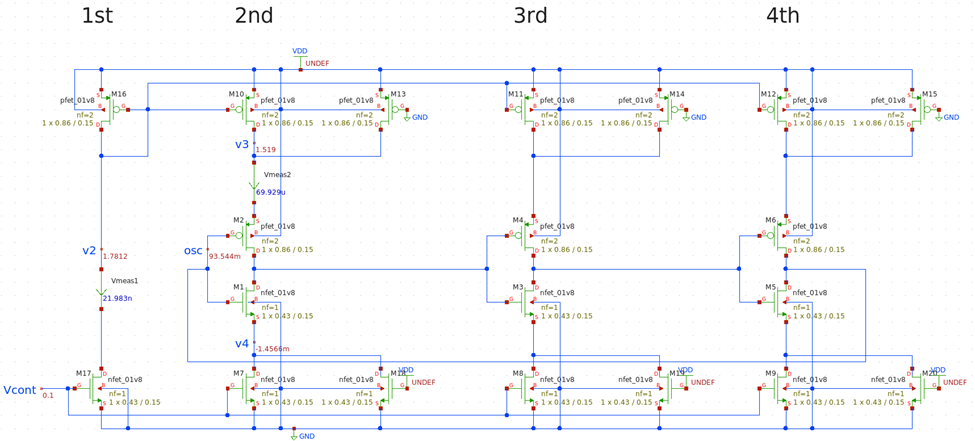
Figure 6 - VCO with on-resistors
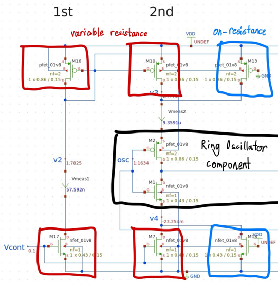
Figure 7 - VCO Functionality
Improving Kvco Linearity
Observation
A linear Kvco is required within the operating control voltage range (0V to 1.8V). Currently, the Kvco slope increases rapidly as V_CONT rises, due to the PMOS growing stronger.
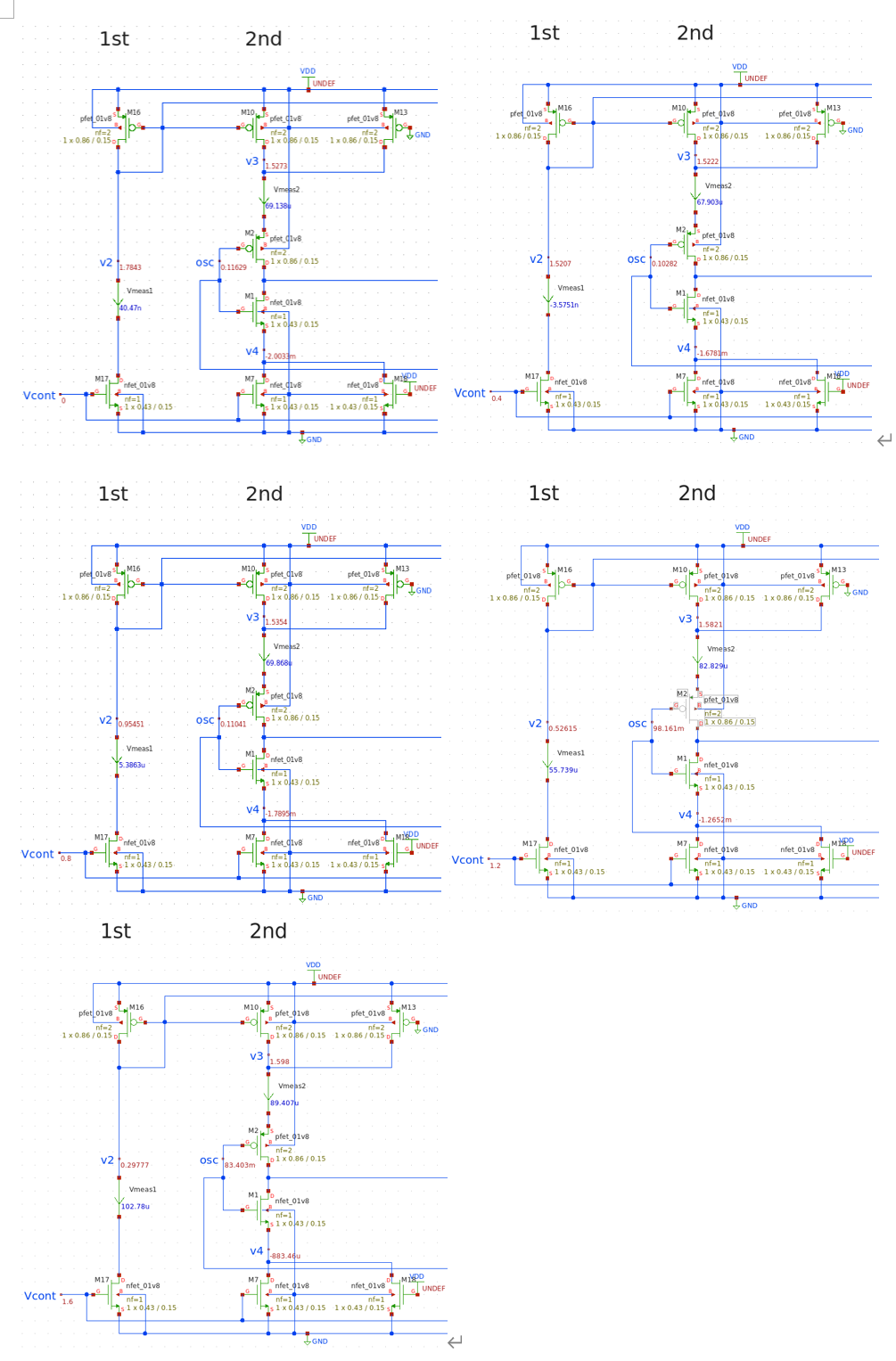
Figure 8 (Click the photo to see the V2 node voltage)
Solution
To moderate the Kvco slope:
Increase the length of the PMOS variable resistance.
But before we do that, we first raise the aspect ratio for both the NMOS and PMOS variable resistance simultaneously for a more dramatic effect.
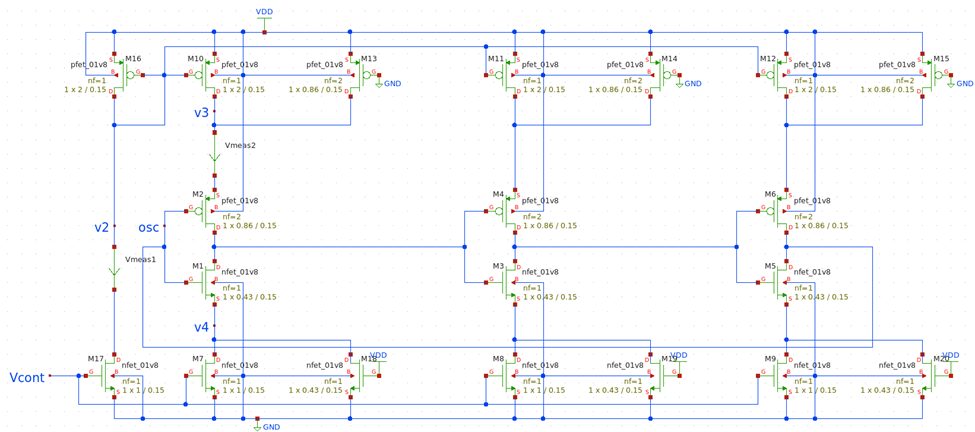
Figure 9 - VCO with increased aspect ratio
We then increase the length of the NMOS variable resistance from 0.15um to 1.5um. The value is set until we find a Kvco plot as figure 10.b. This is a time consuming process to find the appropriate length.
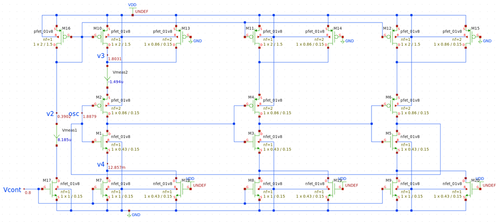
Figure 10.a - VCO with increased PMOS length
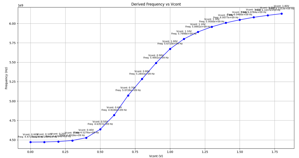
Figure 10.b - Kvco
VCO Configuration
To configure the VCO for the target frequency:
- Increase the length of the ring oscillator transistors from 0.15um to 0.27um.
- Tune the width, if necessary.
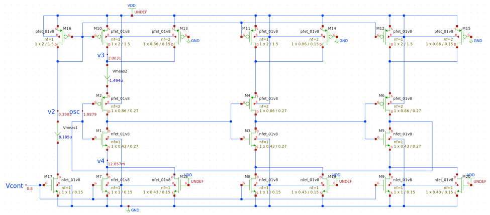
Figure 11.a - VCO
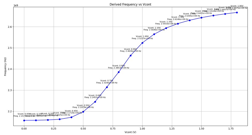
Figure 11.b - Kvco
The process is time-consuming but results in the desired frequency response:
- Kvco Value: 281 MHz/V

- Kvco Max Value: 763 MHz/V

Acutal Design Considerations
However, there are actual design considerations that need to be taken into account.
Looking at Figure 11.a, our VCO’s oscillation relies on the parasitic capacitances in each inverter stage. Also, the VCO only has the minimum three inverter stages, which makes it susceptible to additional parasitic capacitances.
The actual problem arises when the frequency divider is connected to the VCO. In Figure 12, we connected our VCO with the “Divide-by-120” frequency divider (FD). The actual FD design will be covered later on.
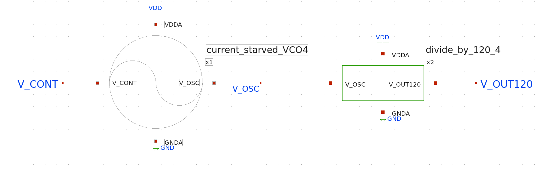
Figure 12
Kvco Measurement with Frequency Divider
Then, if we measure the Kvco of this topology, it appears as Figure 13.
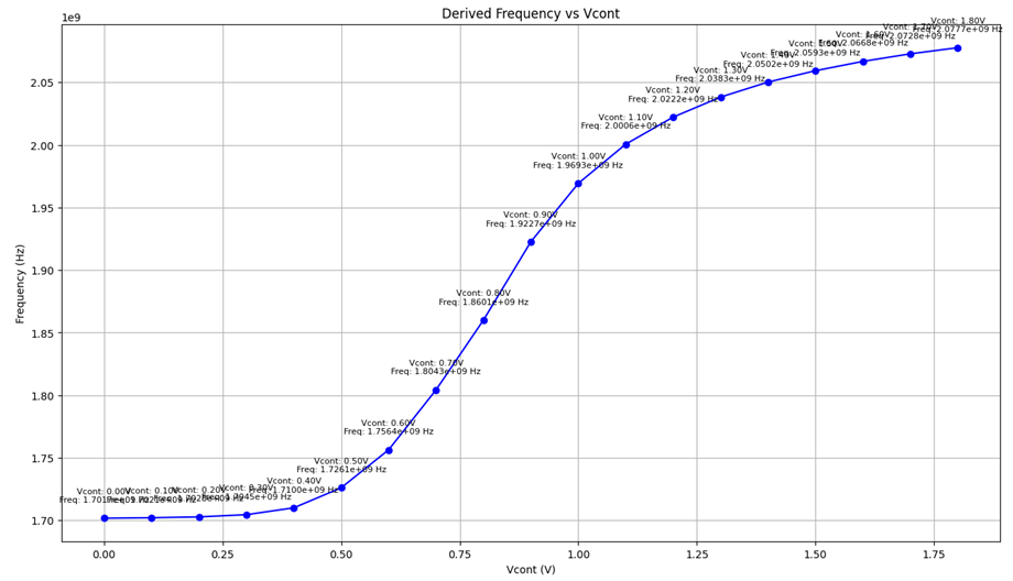
Figure 13
We now see that our VCO output frequency range is entirely out of the target frequency, 2.4GHz.
As a solution, we make the transistor length in the ringed-oscillator shorter, 0.27um to 0.22um.
After that, our new Kvco plot will look like Figure 14.
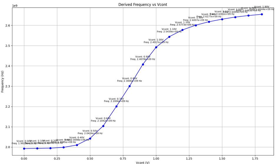
Figure 14
Final Kvco Calculation
Calculating the exact frequency from the raw files, the Kvco value is 362 MHz/V, and this will be our final Kvco value.
Summary and Next Steps
With the Kvco recalculated and adjusted to the desired range, we can now proceed to design the next stages of the PLL, ensuring all design parameters align with the target specifications.
Discussion
Comments
Share questions, corrections, or notes through GitHub.