Table of Contents
As mentioned at the beginning of the previous post, this post presents a design with solutions to the problems in the first topology. The two problems were large transistors and non-linear CP operation.
Large transistors were needed because large parameters are less affected by channel length modulation, which is an issue in nanometer transistors. This was critical in the “Mirroring action” of charge pump branches, where the goal is to mirror the same amount of current from the ideal current source branch.
However, this effect of channel length modulation could be mitigated by using operational amplifiers. If the OPAMP has a high gain, it leads to strong feedback in the transistors. In this condition, their operating points could be matched precisely so that they are somewhat relieved from channel length modulation.
1. Concept of the Proposed Topology
The implementation and the simulation configurations follow as shown below.
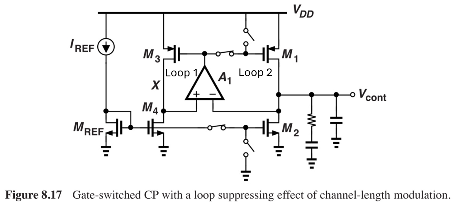
Figure 1. Figure 8.17 from [2]
As we know, if an OPAMP has a high gain, it has the ability to equalize its two differential inputs with strong negative feedback.
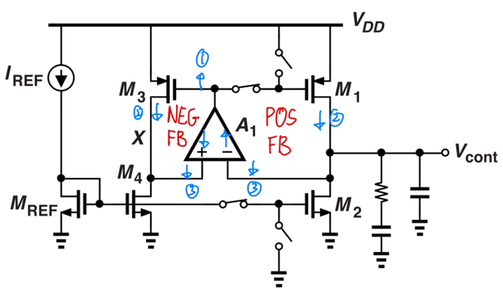
Figure 2
In fig.2, shows the theoretical CP Loop 1, and Loop 2 behavior of negative feedback, and positive feedback, respectively. The circuit also has positive feedback which may not be pleasing for it to work as a bias equalizing branch. However, notice that Loop 2 also consists of switches that depend on PFD output, thus leading to discrete-time behavior, unlike its continuous-time counterpart on Loop 1. While loop 2 is off, it naturally discharges from the succeeding loop filter nodes, and such discharging behavior will also be tracked through the OPAMP since Loop 1 is still engaging in negative feedback. Why is this important? This system allows both M3, M4 branch and M1, M2 branch to hold the same operating point even in nanoscale transistors due to traits of high-gain OPAMP, while M3, M4 is successfully mirroring current from its ideal source, I_REF.
2. DC Analysis
2.1. Topology and Operation Details Regarding DC analysis
The proposed topology is shown in fig.3. The design of the OPAMP will be elaborated in step.2 because its spec requires insights in transient operations. Until then, we assume that the OPAMP has high-gain and therefore the negative-feedback loop keeps its two input the same.
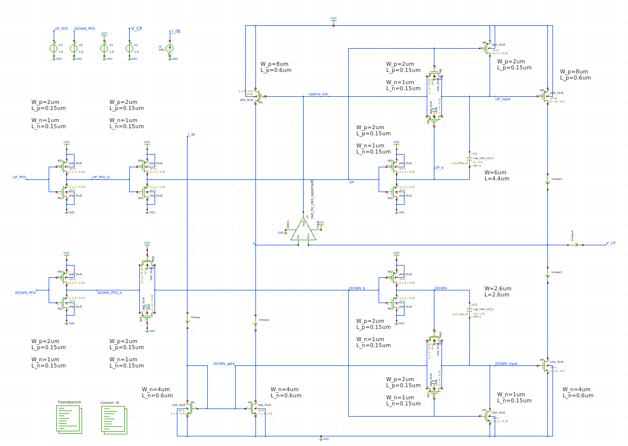
Figure 3
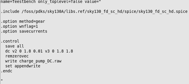
Figure 4
The SPICE code for DC analysis is shown as fig.4, and its result is fig.5.
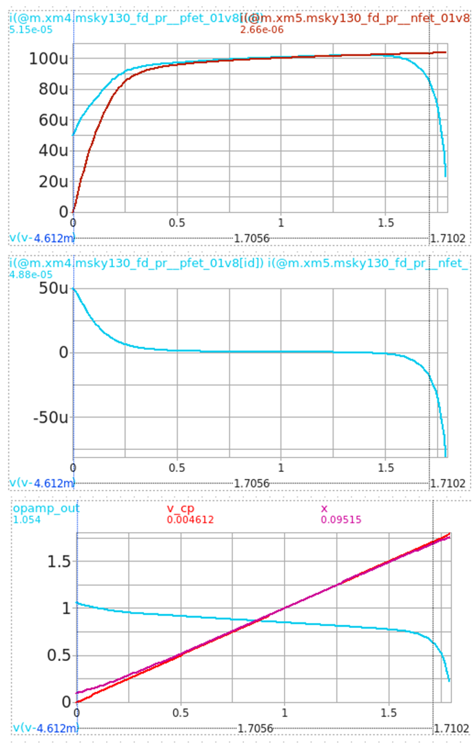
Figure 5
The difference in fig.5. compared to fig.3 from the previous post (for the sake of convenience, it will henceforth be referred to as topology 1) is that the current from UP CP branch steeply decreases as the voltage of node V_CP goes near GND (around 0.25V).
This is because this current mirroring operation works differently from the topology 1. In topology 1, the current is mirrored by connecting the transistor gate of the charge pump branch to the gate of the reference current branches, which has fixed voltages in gate and drain. In topology 2, the reference current has a varying voltage in the gate and drain voltages (both gate and drain for M2, only drain for M3).
For M3, it has fixed gate voltage from the ideal current source with its gate directly connected to the ideal current sourcing NMOS. For its drain voltage, as V_CP voltage changes, node voltage for node X also changes due to OPAMP.
To further examine the voltage-varying operation in node X, we need to discuss M2. As V_CP voltage changes, so does the voltage for node X. To hold this behavior the high gain OPAMP balances the gate of M2 so that node X which is the drain node for “both” M2 and M3 operates and sustains an appropriate drain voltage to mirror 100uA from the ideal current source. This indicates that the common node X of NMOS and PMOS makes them interdependent.
Moving on, as node voltage X falls near GND, it pushes M3 to deep triode region, making it a mere On-resistor. The following situation could be explained through an example as fig.6. When this happens, as node X goes towards GND, and M3 holds resistance such as 5000 ohms. It could only flow 20uA amount of current through the branch, which is far less than 100uA. Thus, to match this decreasing current behavior, the OPAMP increases its output voltage near the threshold voltage.
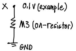
Figure 6
This is also the reason why in essence the node voltage X could not exactly reach GND (0V), which is an interesting property that will also be discussed in step 2. For the sake of convenience in further analyses, I quote this as “Non-convergence to GND”
2.2. Transistor Size Reasoning
| Transistor (Superset) |
Role | Transistor (Subset) |
Role | Sizes (respectively) | Size Reasoning |
|---|---|---|---|---|---|
| M1 | Ideal current source | W = 4um, L = 0.6um | Minimum length to avoid channel length modulation with this OPAMP specs |
||
| M2, M3 | Ideal current source mirroring branch | M2 | Ideal current mirroring for UP operation | W = 8um, L = 0.6um | Minimum length to avoid channel length modulation with this OPAMP specs |
| M3 | Ideal current mirroring for DOWN operation | W = 4um, L = 0.6um | |||
| M4, M5 | Charge pumping current branch | M4 | UP charge pumping operation | W = 8um, L = 0.6um | |
| M5 | DOWN charge pumping operation | W = 4um, L = 0.6um | |||
| M6, M8, M9 | UP switch | M6 | UP charge pump disabling switch | W = 2um, L = 0.15um | Minimum size to ensure minimum slew rate |
| M8, M9 | UP charge pump enabling complementary switch |
W = 2um, L = 0.15um, W = 1um, L = 0.15um |
|||
| M7, M10, M11 | DOWN switch | M7 | DOWN charge pump disabling switch | W = 1um, L = 0.15um | |
| M10, M11 | DOWN charge pump enabling complementary switch |
W = 2um, L = 0.15um, W = 1um, L = 0.15um |
|||
| M12, M13, M16, M17, M20, M21 |
Inverting stage for PFD UP output | M20, M21 | UP signal inverting section for switch actions | W = 2um, L = 0.15um, W = 1um, L = 0.15um |
|
| M12, M13, M16, M17 |
Additive inverters to match overall inverting action |
||||
| M14, M15, M16, M17, M22, M31 |
Non-Inverting stage for PFD DOWN output | M20, M21 | DOWN signal inverting section for switch actions | ||
| M14, M15 | Additive inverter to match overall non-inverting action |
||||
| M18, M19 | Additive pass-gate to match overall non-inverting action |
||||
| C1, C2 | Feed-forward capacitor | C1 | M4 Feed-forward capacitor for better pulse behavior (as a Rect signal) |
W = 6um, L = 4.4um | Appropriate capacitance sizing ensuring 100uA supply |
| C2 | M5 Feed-forward capacitor for better pulse behavior (as a Rect signal) |
W = 2.6um, L = 2.6um |
Table 1. CP Transistor Size Reasoning
Before moving on to an in-depth explanation, table 1 simplifies size reasoning making every other reasoning clear except M1, M2, M3, M4, and M5.
As we have discussed, the current sourcing operation is interdependent between its PMOS and NMOS (M2 & M3 for reference current branch and M4 & M5 for charge pumping branch). As the usual rule of thumb, we normally set the aspect ratio 2:1 for PMOS: NMOS to match the driving force of the transistors. While the length stays in nanoscale, the width is set through trials and errors to find the appropriate size.
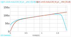
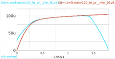
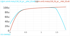
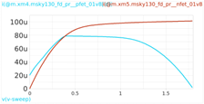
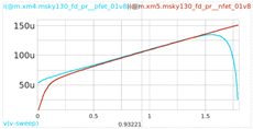
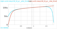
To observe how the operation varies when sized differently, table 2 shows the results.
black;">
Wp = 2um, Lp = 0.15um Wn = 1um, Ln = 0.15um |
Wp = 2um, Lp = 0.3um Wn = 1um, Ln = 0.3um |
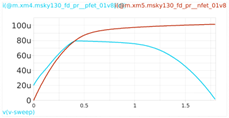
Wp = 2um, Lp = 0.6um Wn = 1um, Ln = 0.6um |
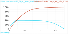
Wp = 2um, Lp = 1.2um Wn = 1um, Ln = 1.2um |
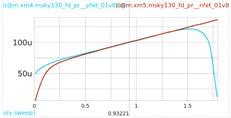
Wp = 4um, Lp = 0.15um Wn = 2um, Ln = 0.15um |
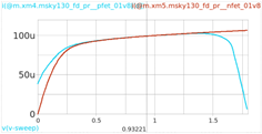
Wp = 4um, Lp = 0.3um Wn = 2um, Ln = 0.3um |
Wp = 4um, Lp = 0.6um Wn = 2um, Ln = 0.6um |
Wp = 4um, Lp = 1.2um Wn = 2um, Ln = 1.2um |
Wp = 8um, Lp = 0.15um Wn = 4um, Ln = 0.15um |
Wp = 8um, Lp = 0.3um Wn = 4um, Ln = 0.3um |
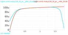
Wp = 8um, Lp = 0.6um Wn = 4um, Ln = 0.6um |
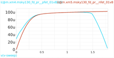
Wp = 8um, Lp = 1.2um Wn = 4um, Ln = 1.2um |
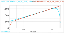
Wp = 16um, Lp = 0.15um Wn = 8um, Ln = 0.15um |
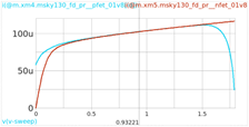
Wp = 16um, Lp = 0.3um Wn = 8um, Ln = 0.3um |
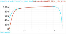
Wp = 16um, Lp = 0.6um Wn = 8um, Ln = 0.6um |
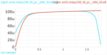
Wp = 16um, Lp = 1.2um Wn = 8um, Ln = 1.2um |
Table 2 . Different Sized Current Mirroring Transistors
While not suffering dramatic consequences from channel length modulation, W_p = 8um, L_p = 0.6um, W_n = 4um, L_n = 0.6um show tolerable outcomes in the smallest widths and lengths. Therefore, it is finally configured as our parameter as in table 1.
3. Transient Analysis
3.1. OPAMP Analysis
Before we begin Transient Simulation of the CP, we must develop our concept of our OPAMP. The priorities are the following.
- Wide range of input common voltage
- High gain
- Unity Gain Bandwidth near 20MHz
- Output impedance
The first factor arises from the concern of our varying V_CONTROL voltage for the VCO which is set as 0~1.8V. To cope with these low to high input common mode voltages, we can develop the concept of rail-to-rail amplifiers.
The second factor is obvious because we need to utilize its feedback property in high-gain conditions. While the exact value is not precisely laid out, we arbitrarily choose the total gain over 50[V/V] as a starting point.
This is because in actual simulations, the output signal of the CP will be shown as fig.7, which somewhat resembles a saw-tooth signal. This is due to the loop filters shown in fig.8, its study is dealt in CH7 in [2] for readers who may be concerned. As we have learned from signals and systems, the Fourier series of a sawtooth signal exhibits decreasing coefficients as the harmonic order increases, emphasizing the significance of the fundamental frequency (20 MHz) as the primary reference. We may consider including higher harmonics such as 40 MHz or more, to ensure a better solution.
The fourth factor was an unexpected priority. The output impedance, or to be more accurate, the capacitance of the output node had to be brought into scope. This was because the output capacitance from the OPAMP 2nd stage and the capacitance of M2 & M4 exacerbated the operation of the CP. Those created unwanted ripples, especially in the first (Slower F_VCO) and third (F_VCO same speed) conditions.
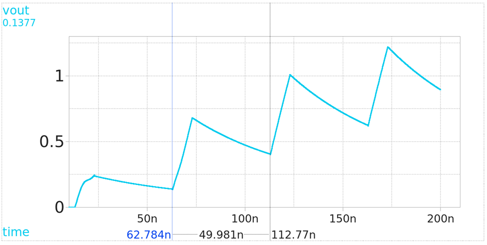
Figure 7. Acutal Transient Response
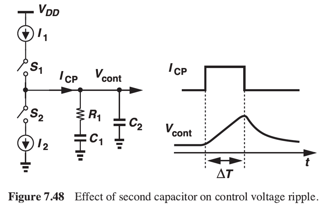
Figure 8. Figure 7.48 from [2]
Moving on to the actual design. We develop the simplest rail-to-rail amplifiers as a starting point.
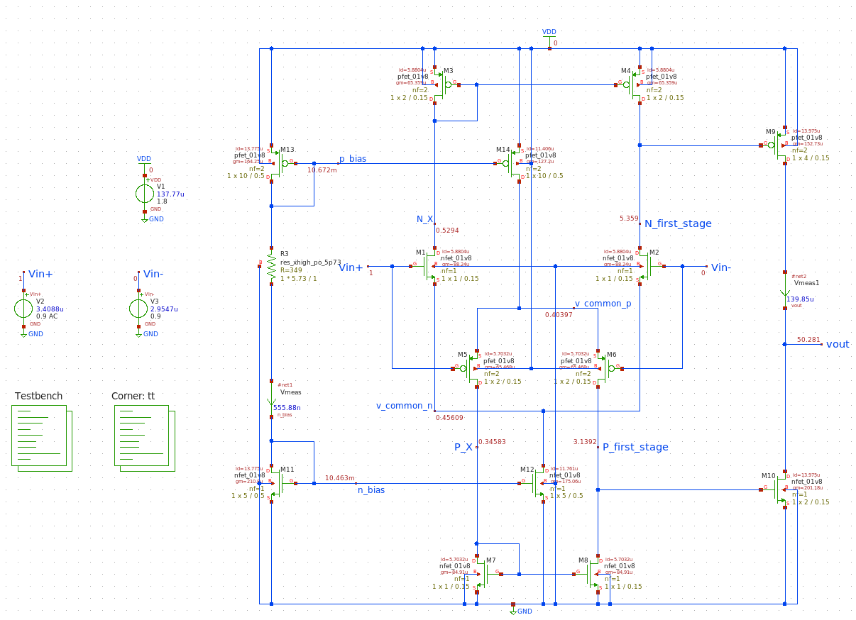
Figure 9. OPAMP Basis Simulation Schematic
Fig.9 is the proposed OPAMP in this CP. Its first stage consists of NMOS and PMOS differential amplifiers with active current mirror load, with current bias from the M13, M11, and R1 branch. The second stage has a PMOS output transistor succeeding the NMOS input stage, combined with its reciprocal pair into a single branch. Note that this is not the most trustworthy OPAMP but get the job done, and table 3 shows the detailed size configurations.
| Transistor (Superset) |
Role | Transistor (Subset) |
Role | Sizes (respectively) | Size Reasoning |
|---|---|---|---|---|---|
| M1, M2, M7, M8 |
1st stage NMOS | M1, M2 | Input NMOS | W = 1um, L = 0.15um | Minimum size in achieving large gain |
| M7, M8 | Active current mirroring NMOS | ||||
| M5, M6, M3, M4 |
1st stage PMOS | M5, M6 | Input PMOS | W = 2um, L = 0.15um | |
| M3, M4 | Active current mirroring PMOS | ||||
| M9, M10 | 2nd stage | M9 | PMOS CS output Stage | W = 4um, L = 0.15um | Appropriate size in balancing both large gain and small capacitive output load |
| M10 | NMOS CS output Stage | W = 2um, L = 0.15um | |||
| M11, M12, M13, M14 |
Current Mirroring Transistors | M11, M12 | Current Mirroring NMOS | W = 10um, L = 0.5um | Minimum length to mitigate significant channel length modulation in this configuration |
| M13, M14 | Current Mirroring PMOS | W = 5um, L = 0.5um | |||
| R3 | Current Biasing Resistor | L = 1um | An arbitrarily chosen value considering layout convenience |
||
| R1, R2 | RHP Zero Cancelling Resistor | R1 | RHP Zero Cancelling Resistor for M9 | L = 1.14um | $ \frac{1}{g_{m_{M9}}} $ value to cancel RHP zero of M9 |
| R2 | RHP Zero Cancelling Resistor for M10 | L = 0.87um | $ \frac{1}{g_{m_{M10}}} $ value to cancel RHP zero of M10 | ||
| CC_1, CC_2 | Miller Compensation Capacitor | CC_1 | Miller Compensation Capacitor for M9 | 1st: W = 8um, L = 8um 2nd: W = 10m, L = 10um 3rd: W = 15m, L = 15um |
Appropriate capacitance sizing regarding the surrounding transistors' sizes, especially M5 |
| CC_2 | Miller Compensation Capacitor for M10 |
Table 3. OPAMP Transistor Size Reasoning
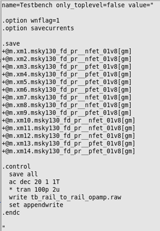
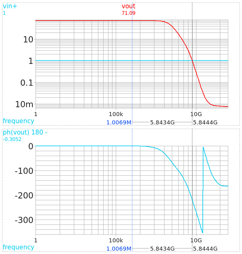
Figure 10. Current Flow in the Third Condition with Revised Transistor Sizes
Fig.10 shows the SPICE code the Bode plot of the OPAMP. It shows that the DC gain is 71 [V/V] , with its unity gain BW as 5.8 GHz. While the OPAMP in this condition is in no good use, we can drive better configuration by applying Miller compensation. By this, the poles in the first and second stages will be split to better stability.
An excellent explanation of this concept is introduced in the youtube link below and it is advisable to watch it before designing this OPAMP.
As the video explains, we can use a resistor to move the right half plane (RHP) zero to infinity, and a capacitor to conduct miller compensation.
As we follow, the value of the resistor at the “p_first_stage” node is chosen precisely as . The value of can be found from fig.9, then the resistor is implemented in the final value of 6514 ohms with a length of 1.14um. The same procedure is conducted for the resistor of the “n_first_stage” node.
The capacitance for the miller compensation could be derived through direct analysis, but such calculation is not recommended due to the difficulty of evaluating every parasitic capacitance in a given topology. In our case, we use equal values for the miller compensation capacitor in both M9 and M10. Then, we alter those values to examine how different capacitance values affect the unity gain BW and transient simulation results.
Fig.11, 12 and table 4 illustrates the traits of the OPAMPs with capacitance variations.
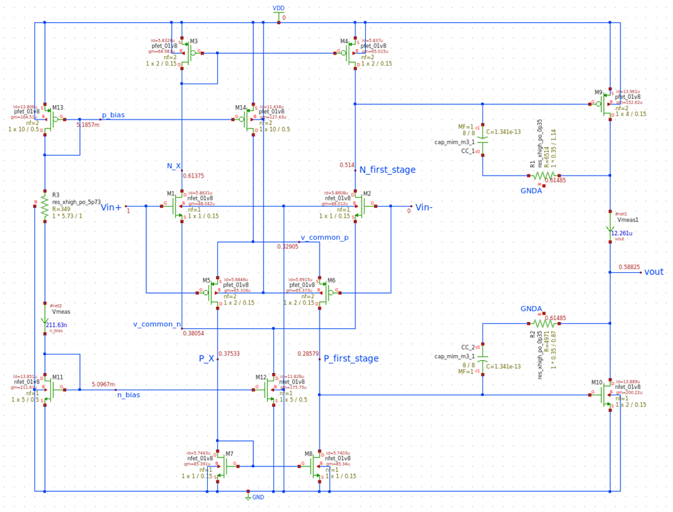
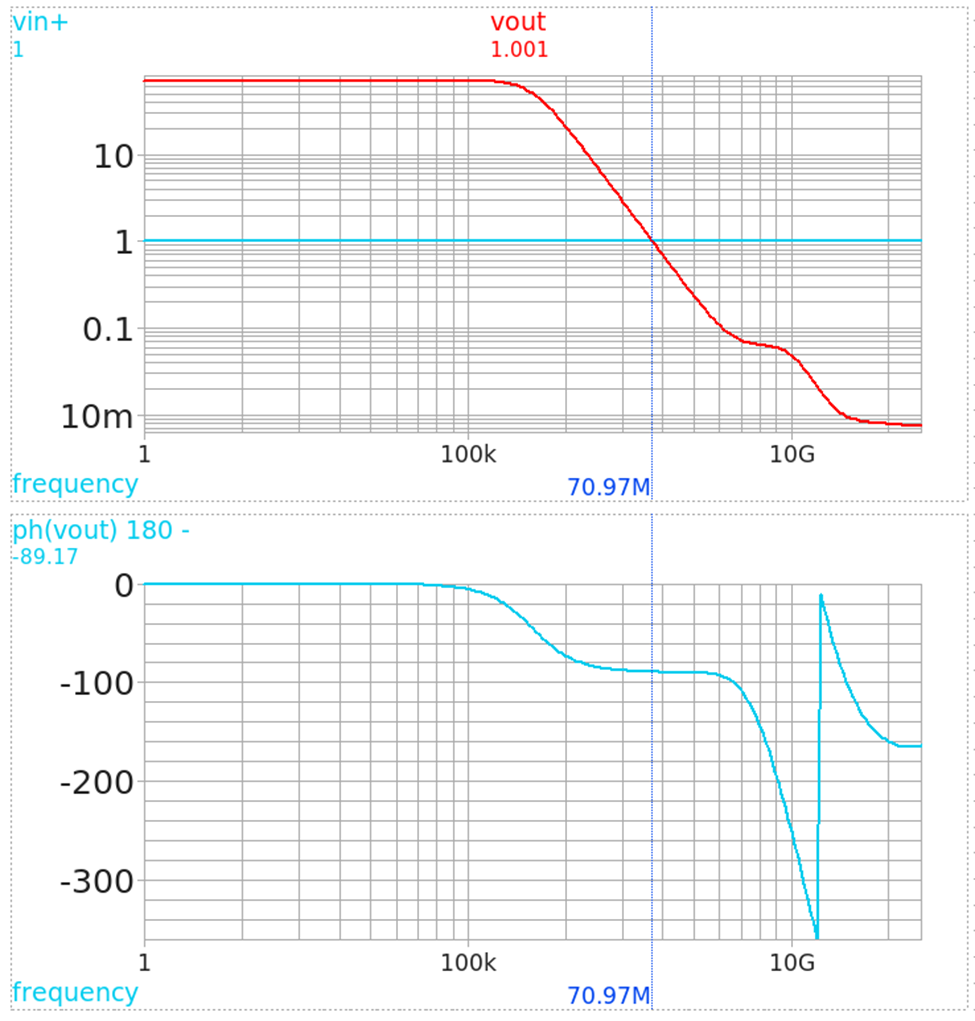
Figure 11. OPAMP Final topology (Left), OPAMP1 Bode Plot (Right)
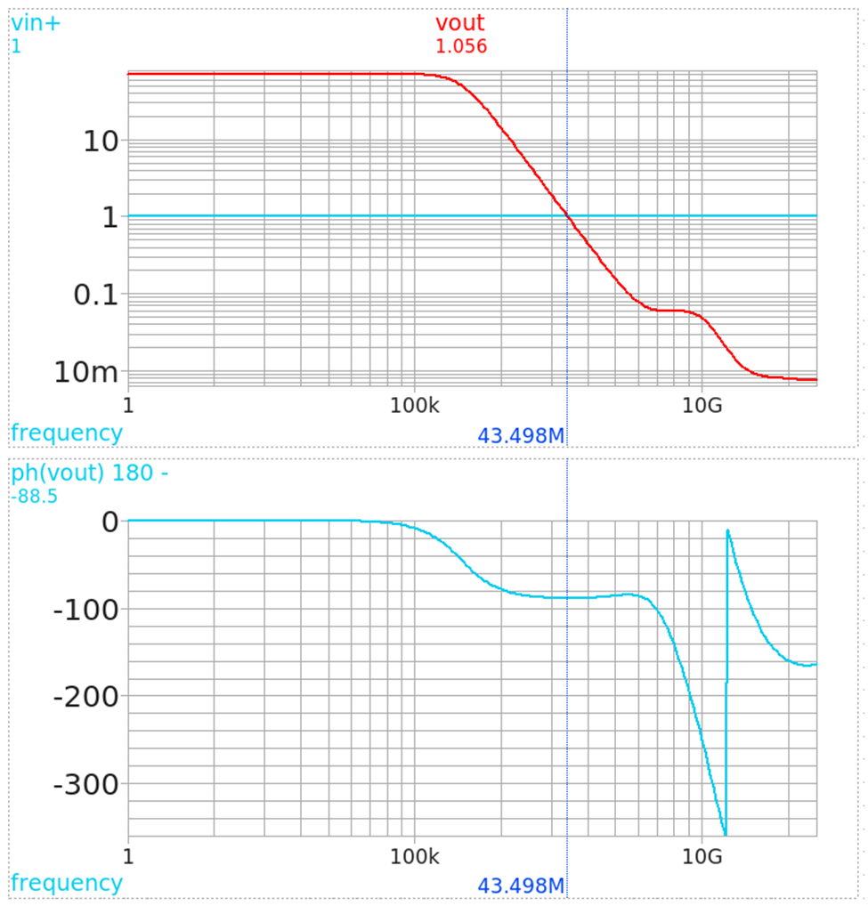
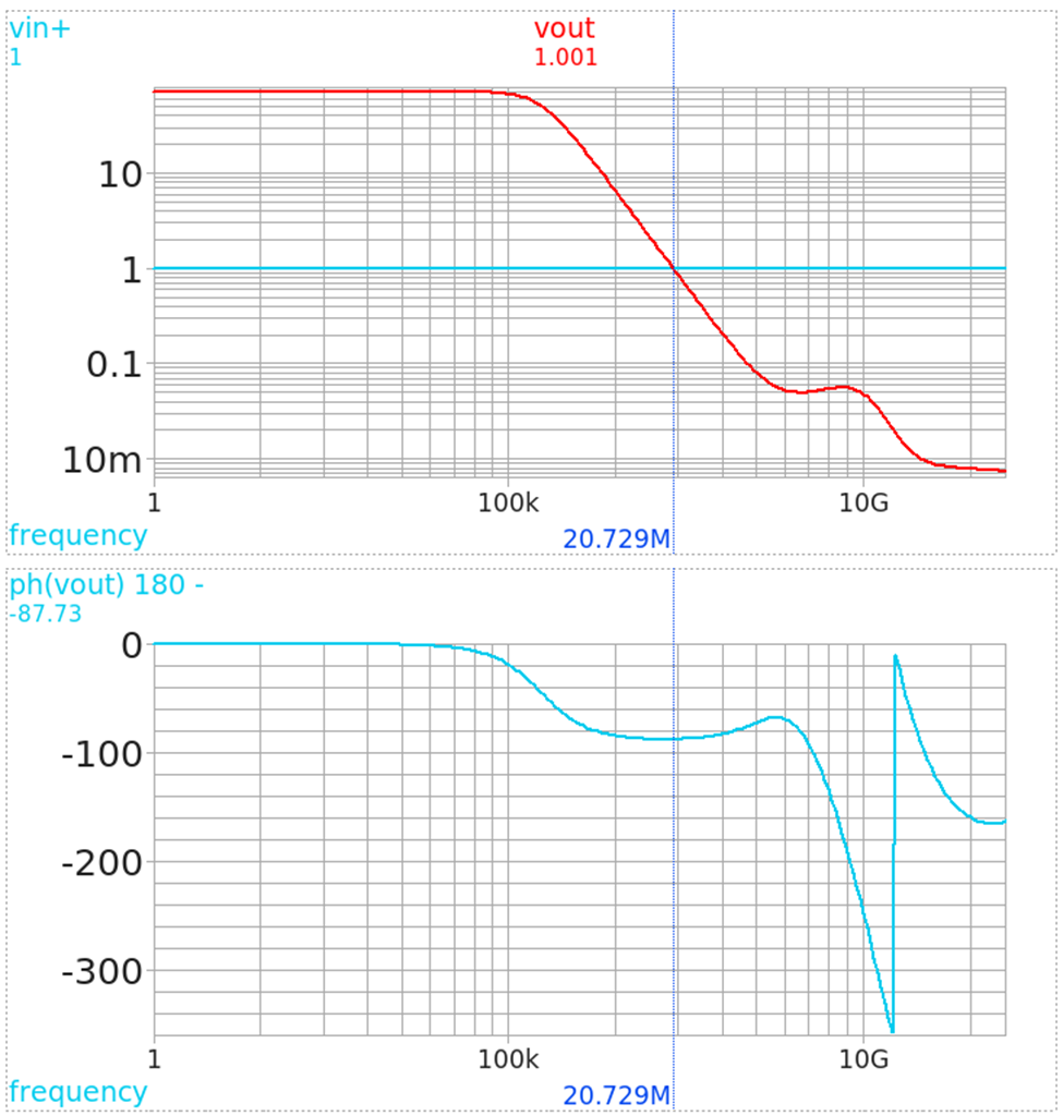
Figure 12. OPAMP2 Bode Plot (Left), OPAMP3 Bode Plot (Right)
| SPECS \ CASES | OPAMP 1 | OPAMP 2 | OPAMP 3 |
|---|---|---|---|
| Size | 8um X 8um | 10um X 10um | 15um X 15um |
| Capacitance | 0.134pF | 0.208pF | 0.461pF |
| Unity gain BW | 70MHz | 44MHz | 20MHz |
Table 4. OPAMPs with different size Miller Cap.
3.2. Testbench Considerations
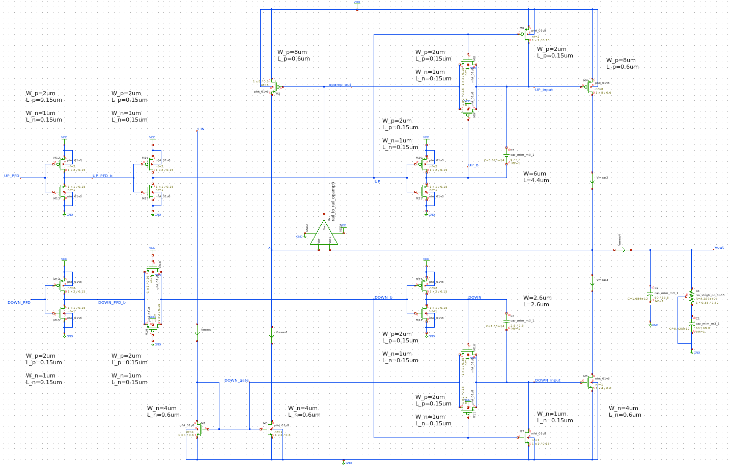
Figure 13. Transient Simulation Schematic
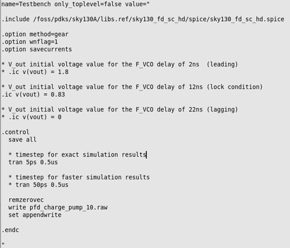
Figure 14. Transient Simulation SPICE
The testbench is similar to the previous post.
3.3. Simulation Results
We test the transient simulation by sorting three cases “Case 1” “Case 2” and “Case 3” The only different component in those cases is the OPAMP, which is denoted in table 4. Then, like the previous post, we examine all three conditions for each case. The 1st condition (F_REF slower than F_VCO), 2nd condition (F_REF faster than F_VCO), and 3rd condition.
1st condition (F_REF slower than F_VCO)
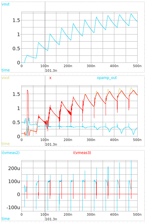
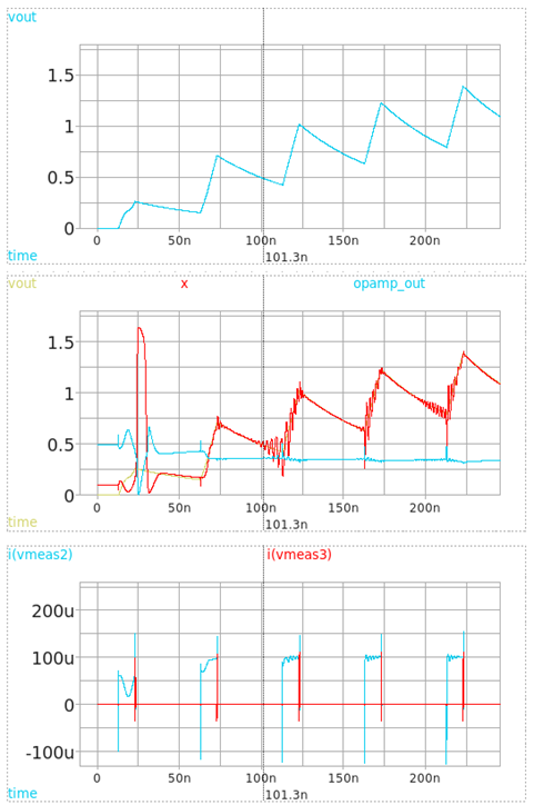
Figure 15. Case 1, Condition 1
2nd condition (F_REF faster than F_VCO)
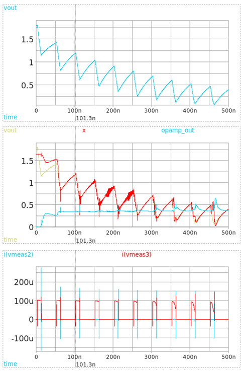
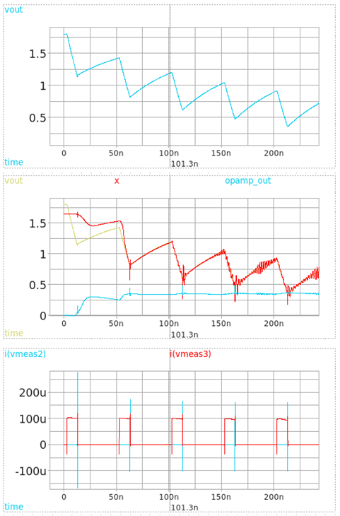
Figure 16. Case 1, Condition 2
3rd condition (F_REF same as F_VCO)
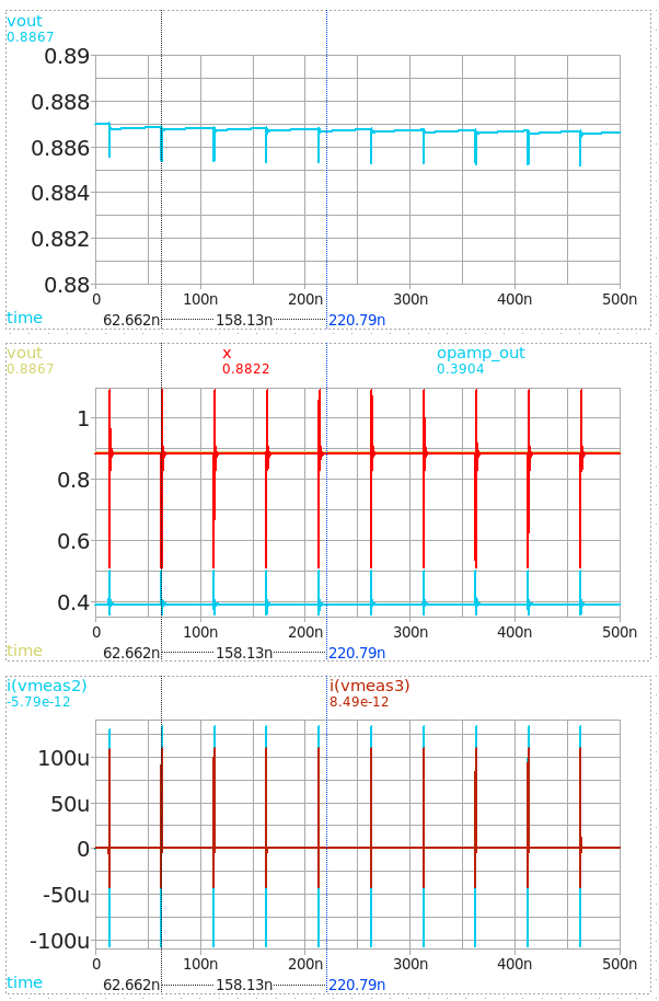
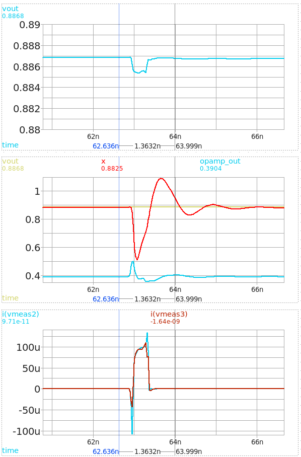
Figure 17. Case 1, Condition 3
1st condition (F_REF slower than F_VCO)
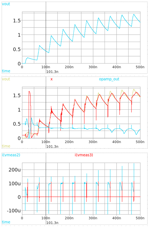
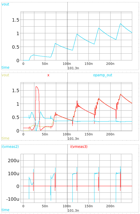
Figure 18. Case 2, Condition 1
2nd condition (F_REF faster than F_VCO)
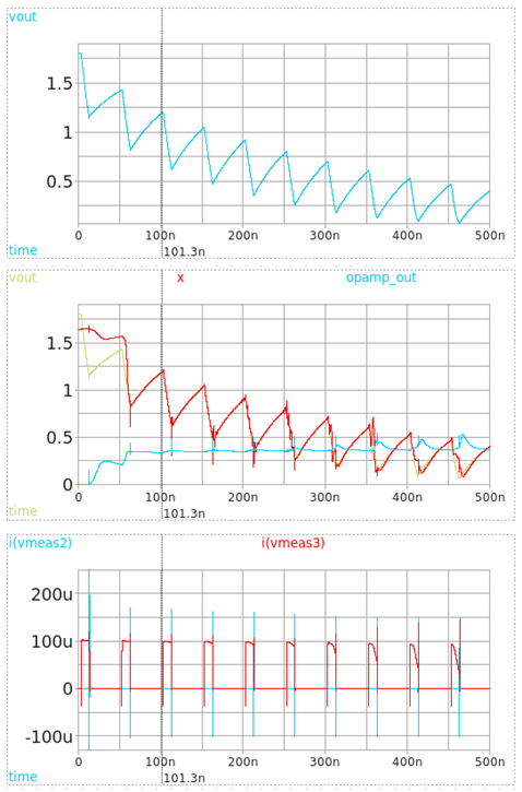
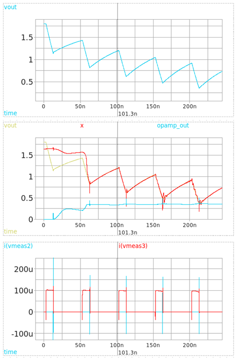
Figure 19. Case 2, Condition 2
3rd condition (F_REF same as F_VCO)
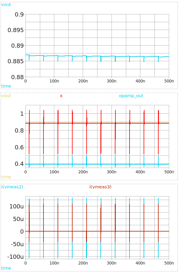
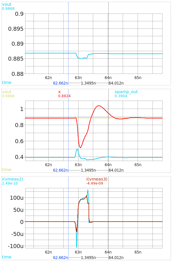
Figure 20. Case 2, Condition 3
1st condition (F_REF slower than F_VCO)
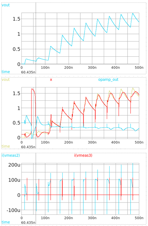
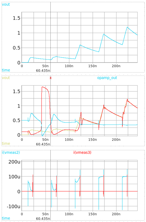
Figure 21. Case 3, Condition 1
2nd condition (F_REF faster than F_VCO)
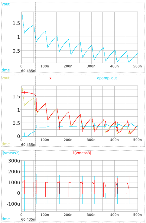
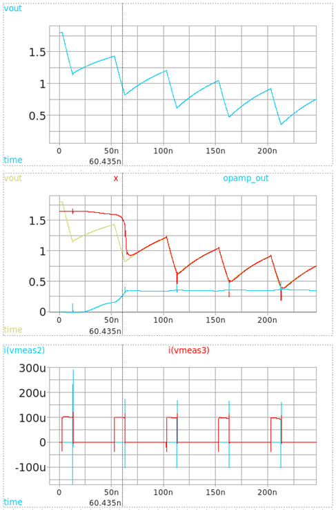
Figure 22. Case 3, Condition 2
3rd condition (F_REF same as F_VCO)
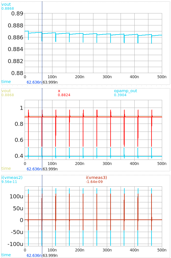
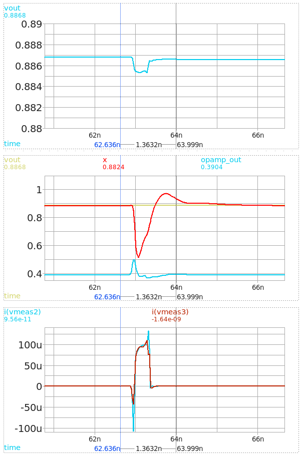
Figure 23. Case 3, Condition 3
The second condition in all three cases shows no issue providing 100uA current. For the third condition, as the capacitance gets bigger, it lowers the unity gain BW and the steady-state responses grow more stable. However, it is the opposite for the first condition. As the unity gain BW gets smaller, the CP suffers from slow coherence between the differential input nodes of the OPAMP, as shown in fig.21.
This shows that if the capacitance of the OPAMP output node is too small, the PLL will suffer from ripples in the lock state. If it is too big, the PLL will suffer from inappropriate charge-pumping actions in the first conditions. Therefore, choosing a moderate-size capacitor such as OPAMP 2 is advisable, which has a unity gain BW of approx. 44MHz.
4. Design Analysis
4.1. Evaluation of Conditions
For better comprehension, there are few notes to discuss, especially the first and the third.
The first conditions require further explanation for comprehension. As shown in fig.5, the reference current branch could only provide 40uA in initial conditions. That is why the CP experiences an insufficient pulse magnitude at the first clock.
Also, all cases show that the CP experiences a sudden surge in node “X” after the first clock. Such behavior occurs from node “X” being non-zero due to “No-convergence to zero.” During the first clock, the negative and positive feedback operate to match the two differential inputs. However, the first clock abruptly ends after 24ns, and the OPAMP is only left with negative feedback with the two differential input node voltages even far apart from the initial status. Thus, the negative feedback loop of the OPAMP lowers its output voltage, which raises the node voltage of X due to the M2 CS stage. Therefore, the CP experiences a sudden surge in the X node.
Second, the third conditions answer the C1, C2 size reasoning back from table.1. It would look like fig.24 in the third condition without the capacitors.
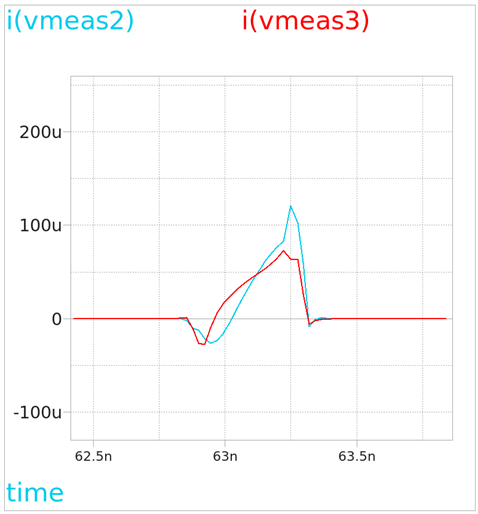
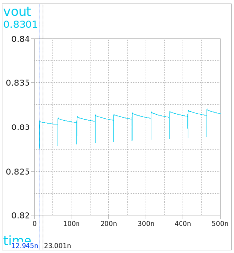
Figure 24. Current (Left), Vout (Right) Aspect before Feedforward Capacitor
The values of C1 and C2 are decided so that both UP and DOWN pulses become rectangular signals of the same 100uA magnitude while outputting a constant output.
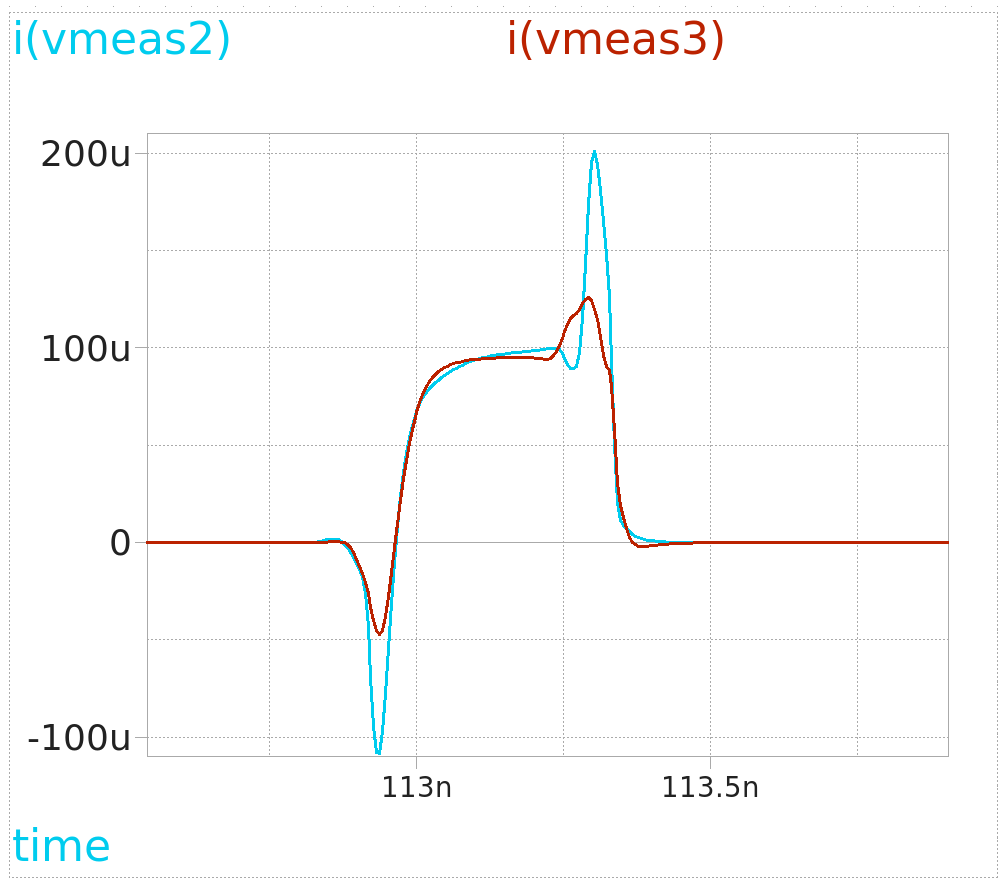
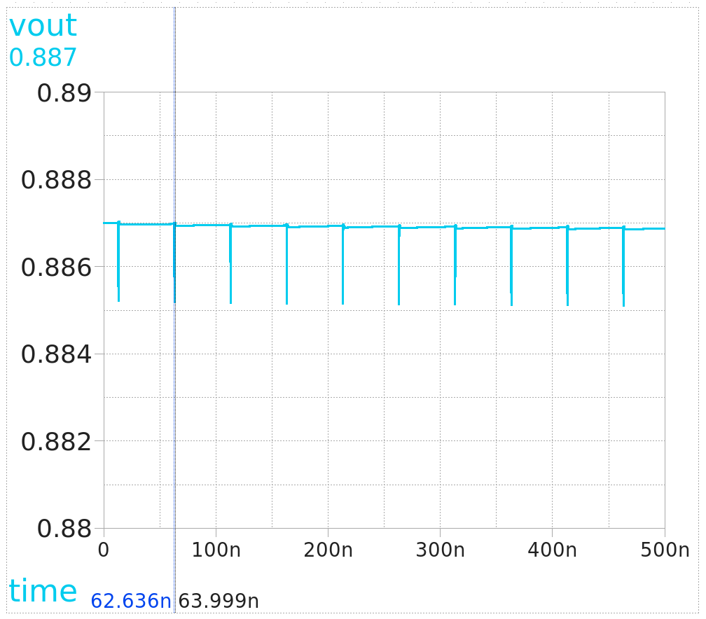
Figure 25. Current (Left), Vout (Right) Aspect after Feedforward Capacitor
4.2. Charge Pump Dead Zone
The dead-zone configuration for this CP is the same as the previous post, and the results are shown in fig.26
Charge Pump Dead Zone Section {: .prompt-info }
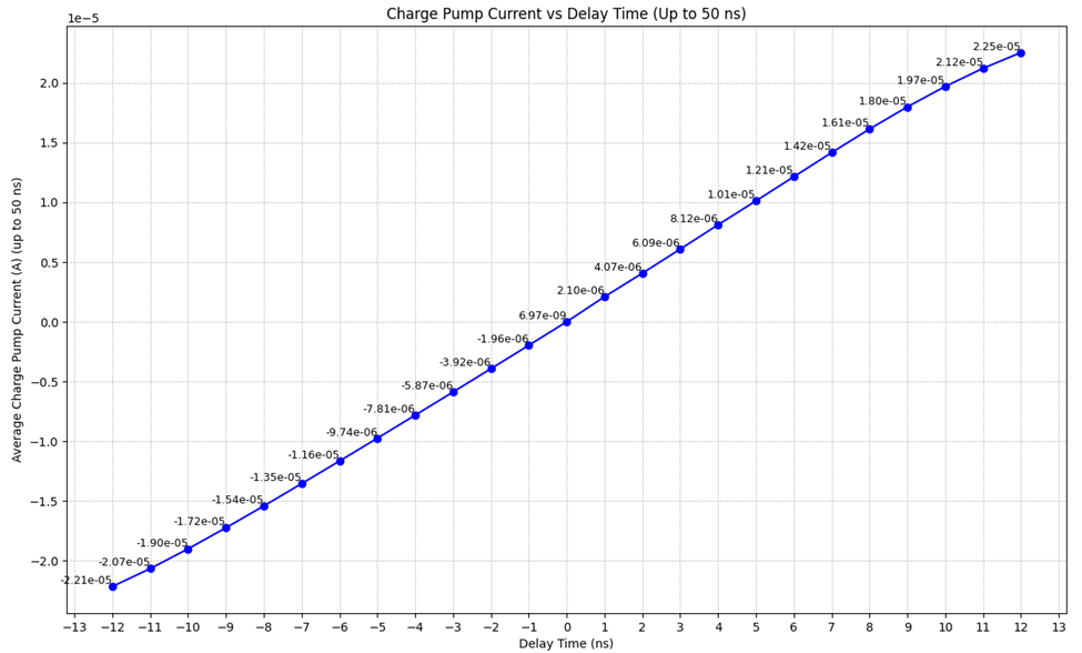
Figure 26. Current VS. Delay Plot
This proves that this CP has linear functionality within nanoscale design. It was possible due to using an OPAMP suppress channel length modulation.
In the next post, a new topology will be suggested in nanoscale design to resolve the above two issues.
References
- [1] Design of Analog CMOS Integrated Circuits, 2nd Edition - Razavi
- [2] Design of CMOS Phase-Locked Loops: From Circuit Level to Architecture Level, 1st Edition - Razavi
Discussion
Comments
Share questions, corrections, or notes through GitHub.