PLL - Design Parameters Part 2: Loop Filter

From the previous post “Voltage Controlled Oscillator Design,” we obtained the Kvco as 362 MHz/V.

Back in the post “Design Parameters Part 1,” we left off $C_1$ , $R_1$ , and Kvco undecided.
Now, with Kvco being set, we move on to the derivation of $C_1$ and $R_1$ .

Loop Filter Derivation

From that post, we specifically decided to start from a 2nd order PLL for the loop filter parameter configuration.

{\scriptstyle H(s)_{\text{closed loop}}} = \frac{\frac{I_p}{2\pi} \cdot \left( R_1 + \frac{1}{C_1 s} \right) \cdot \frac{K_{\text{VCO}}}{s}}{1 + \frac{I_p}{2\pi} \cdot \left( R_1 + \frac{1}{C_1 s} \right) \cdot \frac{K_{\text{VCO}}}{s} \cdot \frac{1}{M}}

Equation 1: 2nd order Closed Loop Transfer Function

This allows us to use control theory to analyze the 2nd-order closed-loop PLL system.

Key Equations

\zeta = \frac{R_1}{2} \sqrt{\frac{I_p K_{\text{VCO}} C_1}{2\pi M}}

Equation 2: Damping Factor

\omega_n = \sqrt{\frac{I_p K_{\text{VCO}}}{2\pi M C_1}}

Equation 3: Natural Frequency

As Eq.3 has just one unknown variable ( $C_1$ ), we will start deriving from the natural frequency.

Discrete-Time Nature of PLL

First, we need to realize that our PLL carries a Discrete-Time (DT) nature. This is because the VCO is driven by the output of the PFD/CP/Loop Filter cascade, which is a ramp response.

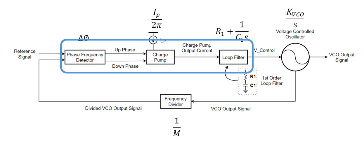
Figure 1: PLL and the Highlighted PFD/CP/Loop Filter Cascade

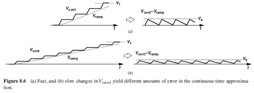
Figure 2: Ramp Response Signal of the PFD/CP/Loop Filter Cascade

This discrete nature interferes with our attempt to view the PLL as a continuous system. However, as shown in Figure 2(b), if we were to state the changes slowly, we can approximate back the system to be a continuous system. By then, the analysis through transfer function gains some reliability.

A rule of thumb to ensure this slow change in the loop is to select the loop bandwidth approximately equal to 1/10 of the input frequency.
We know our input frequency (f_REF) as 20 MHz, thus the loop bandwidth has to be 2 MHz.

Open Loop Bandwidth Selection

But which bandwidth? $\omega_{-3dB}$ (3dB cutoff bandwidth of the Closed Loop System) or $\omega_u$ (unity-gain bandwidth of the Open Loop System)?

H(s)_{\text{Open Loop, Fig.1}} = \frac{I_p}{2\pi} \cdot \left( R_1 + \frac{1}{C_1 s} \right) \cdot \frac{K_{\text{VCO}}}{s}

Equation 4: Open Loop Transfer Function

If this still raises concerns, we can take further validations.

Say we set the 2nd order system to have a damping factor ( $\zeta$ ) of 1, it shows as the figure below.
In such ( $\zeta = 1$ ) configuration, it shows the relationships of the bandwidths as $\omega_{-3dB} \approx 2.5\omega_n$ , and $\omega_u \approx 2.1\omega_n$ .
By this, the two bandwidths are close in values, which means that even if we choose $\omega_{-3dB}$ over $\omega_u$ , we can still expect the similar results.

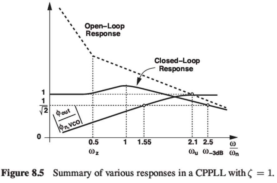
Figure 3: Various PLL Response

\frac{\omega_{REF}}{10} = \omega_u = 2.1 \omega_n

Equation 5: Relationship of Reference, Unity-Gain, Natural Frequency

Deriving C1 and R1

Calculating C1

\frac{2\pi \times (20 \, \text{MHz})}{10} = \omega_n = 2.1 \sqrt{\frac{I_p K_{\text{VCO}}}{2\pi M C_1}}

\frac{2\pi \times (20 \times 10^6)}{10} = 2.1 \sqrt{\frac{(100 \times 10^{-6}) \times (2\pi \times 362 \times 10^6)}{2\pi \times 120 \times C_1}}

C_1 = (2.1)^2 \times \frac{(100 \times 10^{-6}) \times (2\pi \times 362 \times 10^6)}{2\pi \times 120 \times \left( \frac{2\pi \times (20 \times 10^6)}{10} \right)^2}

C_1 \approx 8.42pF

Equation 6: C1 Derivation

Therefore the value of $C_1$ = 8.42pF, and the value of $C_2$ taken as 1/5, which will be roughly $C_2$ = 1.68pF.

Configuring $C_1$ we can move on to the configuration of the $R_1$ value. As we set the damping factor ( $\zeta$ ) as 1, the calculation starts from Eq.2 as below.

Calculating R1

\omega_n = \sqrt{\frac{I_p K_{\text{VCO}}}{2\pi M C_1}}

1 = \frac{R_1}{2} \sqrt{\frac{(100 \times 10^{-6} \, \text{A}) \times (2\pi \times 309 \times 10^6) \times (7.19 \times 10^{-12})}{2\pi \times 120}}

Equation 7: R1 Derivation

In conclusion, we have $R_1$ = 42.9kΩ.

Simulation in MATLAB

We validate these values using MATLAB Simulink and the Control System Designer.
Below are the Design Parameters and the Simulink diagram:

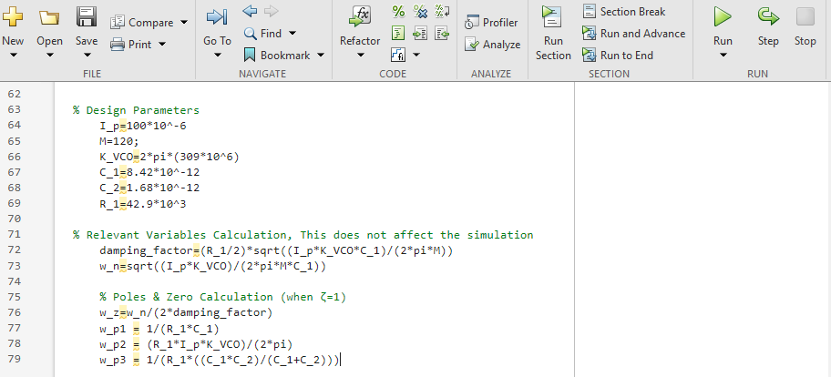
Figure 4: Design Parameters for PLL

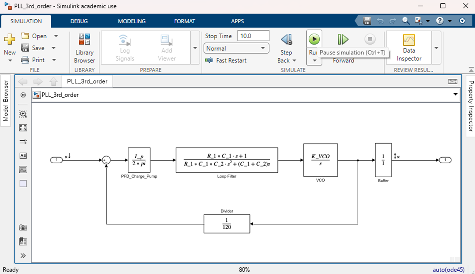
Figure 5: Simulink Diagram for PLL

This represents our target topology that we mentioned in “PLL Design Parameters: Part 1”

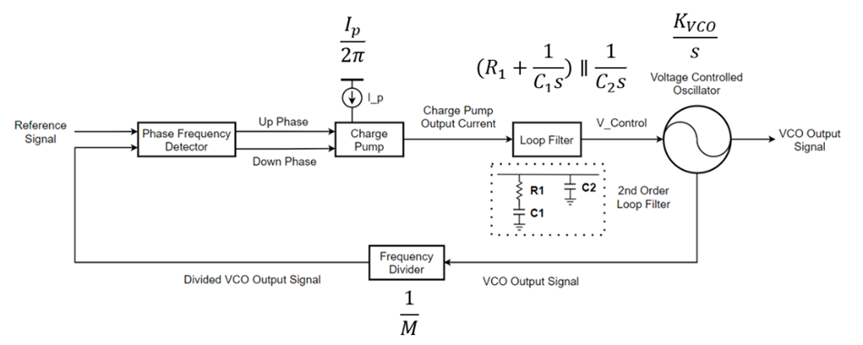
Figure 6: PLL Circuit Representation

Evaluating the results through “Control System Designer App” in simulink will look like this.

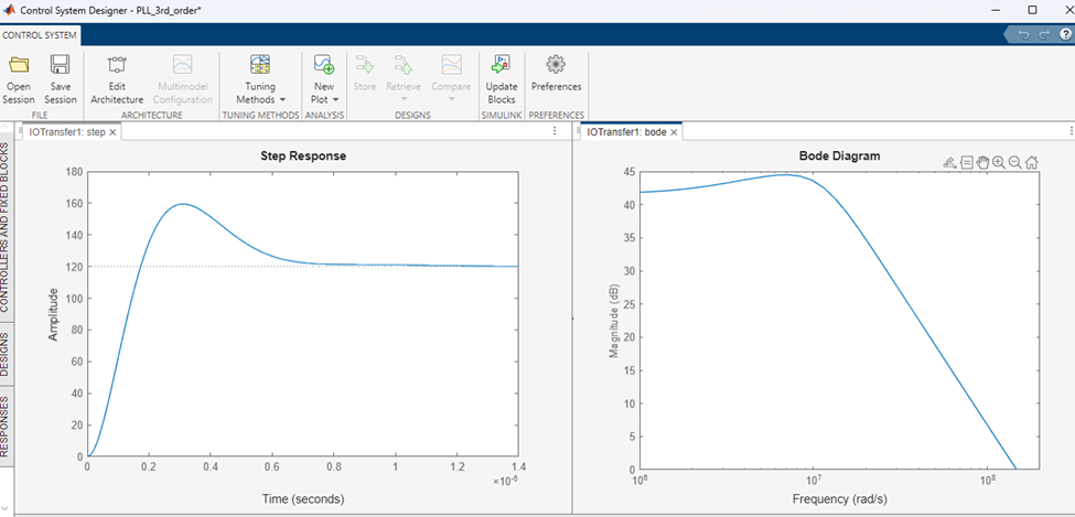
Figure 7: Step Response, Bode Plot

Xschem Implementation

Finally, in Xschem, the schematic looks like this:

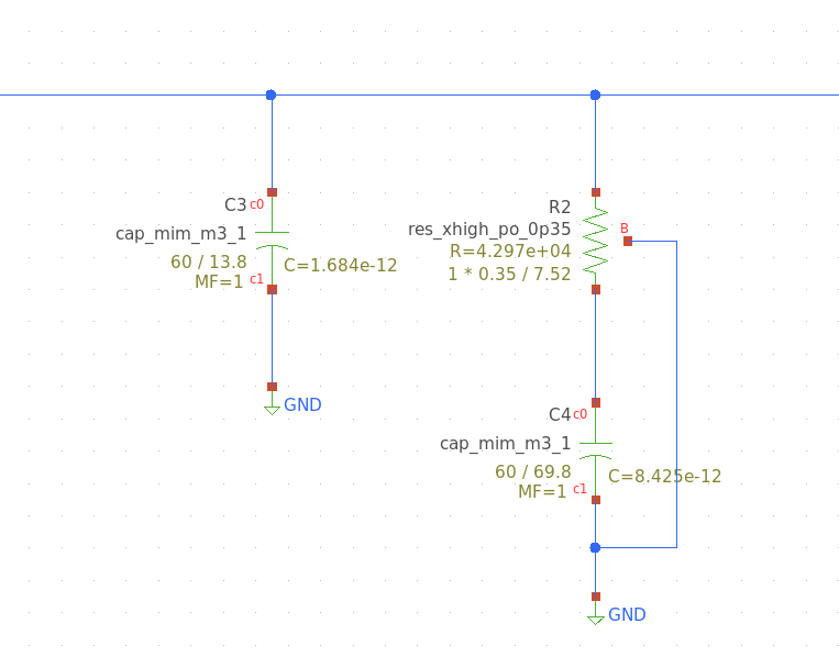
Figure 8: Xschem Implementation

With the loop filter parameters derived and simulated, we finished the design parameter configuration. We can now move on to Phase Freqeuncy Detector (PFD) design in the next post.