Table of Contents
We now begin our design in charge pumps (CP). In this section, I divided the topics into two posts. This post presents the first CP design in the simplest topology but with limitations. The next post will propose the second CP that provides solutions to the first design while designed in nanoscale topology.
When designing the CP, there are two priorities. First, the design must guarantee that it supplies 100uA along the V_out DC sweep among the operating V_CONT range (0V ~ 1.8V). Second, the actual transient response of the charge pump must be inspected.
1. Concept of the Proposed Topology
Beginning the analysis of the first CP design, the topology is shown below.
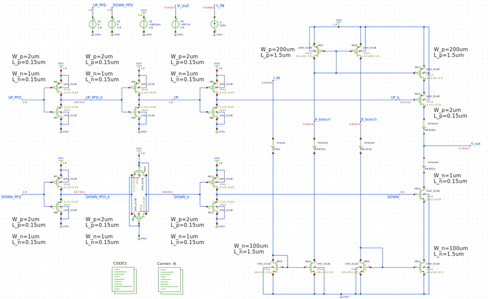
Figure 1
In fig.1, M1~M6 are the pulse inverting stages for charge pump (CP) PMOS input, and M7~M12 are the pulse non-inverting stages for CP NMOS input. Some might think this could be done by adding a single inverter on the PMOS input, but such configuration can bring timing mismatches for the PMOS and NMOS input.
To mitigate that effect, M9, M10 are added as pass-gates for the non-inverting stage. Compared to the inverters, however, this pass-gate is comprised of mismatch due to large parasitic capacitance. This could be resolved to some extent by placing it in the middle of two inverters as fig.1.
For size considerations, the pulse inverting and non-inverting stages (M1~M12) are implemented in the smallest dimensions possible, so they do not suffer from excessive parasitic capacitance from the device. This concept is also applied to the CP input PMOS and NMOS (M13~M14) so their impedance does not hinder the loop filter components. However, these two transistors were not pushed to their minimum size limit (PMOS [W:0.86um, L:0.15um], NMOS [W:0.43um, L:0.15um]), because such configuration could bring current mismatch.
M15~M17 are the PMOS current mirror stages and M18~M21 are the NMOS current mirror stages. For size considerations, they are implemented in big dimensions so that the role of current mirroring is not degraded due to channel length modulation.
2. DC Analysis
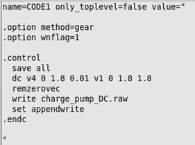
Figure 2
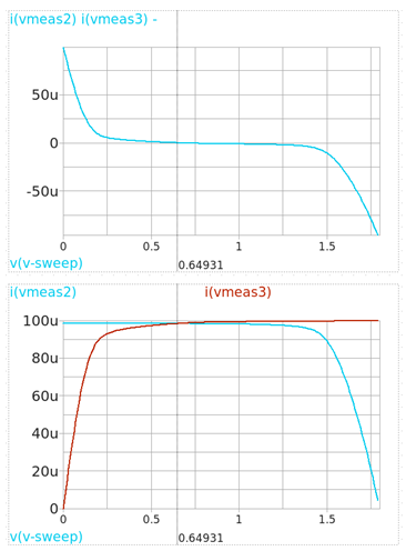
Figure 3
Fig.2 is the spice code for the DC sweep simulation, and the plots in fig.3 are the results. We find out that the proposed CP provides 100uA in the operating V_CONT ranges.
3. Transient Analysis
3.1. Testbench Considerations
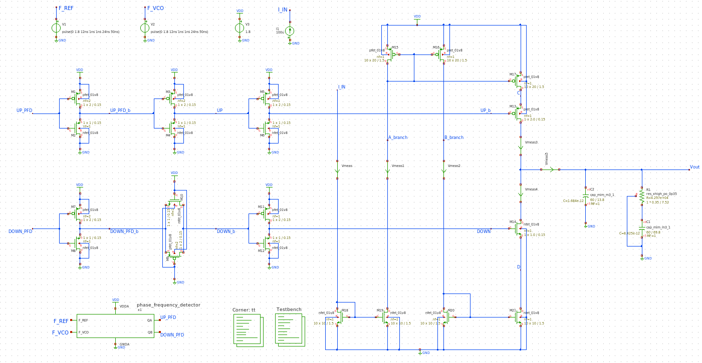
Figure 4
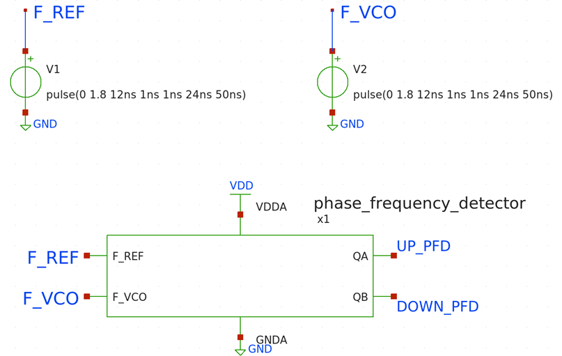
Figure 5
Apart from fig.1, CP is now connected with the PFD and the loop filter components. The input F_REF and F_VCO pulses are shown in fig.5, along with the PFD that we created from the previous post. The delays of pulse signals in F_REF and F_VCO are both set as 12ns. By altering the delay value of F_VCO, we can test conditions where F_VCO is “slower”, “faster” and “same speed” to F_REF.
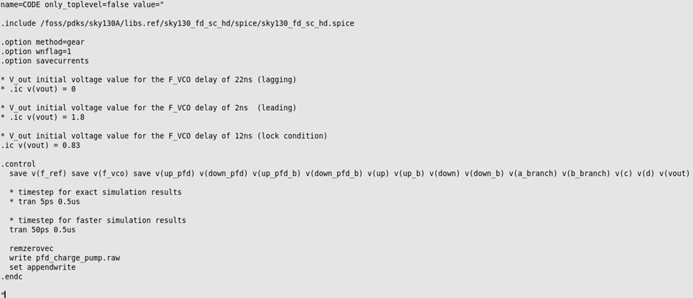
Figure 6
Fig.6 is the SPICE code for the transient response simulations with some comments explaining some of the code lines. The reason for choosing timesteps 50ps and 5ps is related to the validation of unwanted oscillations. In simulations, the rule of thumb for selecting the appropriate timesteps is to choose a 1/10 value, and our frequency of interest is the reference frequency, which is 20MHz, 5x10⁻⁸ s (50ns). Thus, we could choose a timestep of 5ns. However, to further validate for possible oscillations that could arise from amplifications in parasitic capacitances, smaller timesteps 50ps and 5ps were chosen.
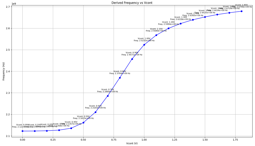
Figure 7
0.8 + \left( \frac{ \text{2.4 GHz} \space - \space \text {Frequency of 0.8V VCO}}{\text {Frequency of 0.9V VCO} - \text {Frequency of 0.8V VCO}} \right) \cdot \text {V_cont Step Size}
Equation 1: V_cont Derivation
The V_CONT value for when the F_REF and F_VCO have the same speed are derived as fig.7. Where 0.8V exerts 2.37GHz and 0.9V produces 2.46GHz, we assume Kvco is linear between these two points and derive the V_CONT value where the VCO can produce 2.40GHz output signal. After the derivation, we configure the initial V_out voltage to 0.83V.
3.2. Simulation Results
1st condition (F_REF slower than F_VCO)
Fig.8 is the pulse response of this transient response. The plots on the left show the full picture, and the plots on the right show the close-up pulses. The notation on the top margin of each plot depicts which node signal they are showing. The plots are orderly put from the PFD output to the CP branch input.
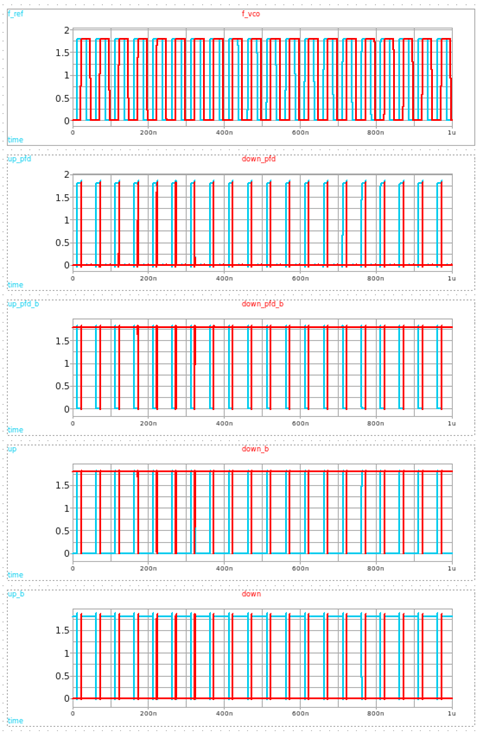
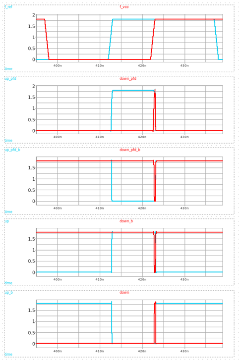
Figure 8. Input Pulse signals of the First Condition
Starting from the top, fig.9 shows the plot of PMOS and NMOS current of the CP / M13 & M14 / M17 & M21 / the (PMOS current - NMOS current) which is the current provided to the loop filter / and finally the V_out, respectively.
The 4th row from fig.9 shows that the CP is providing a little more than 100uA, this due to the charge injection from the parasitic capacitance from the big MOSFETs.
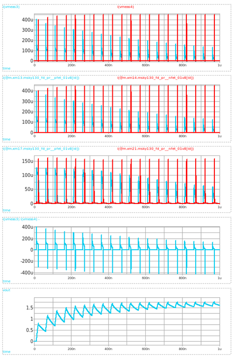
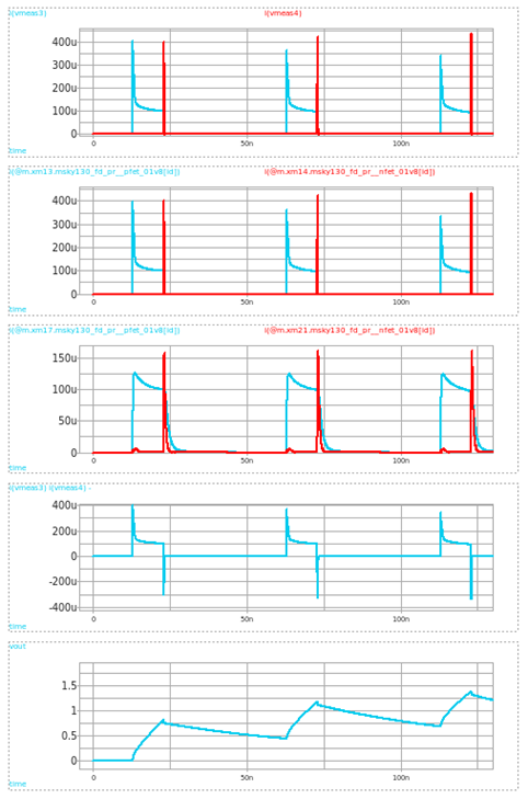
Figure 9. Current Flow in the First Condition
2nd condition (F_REF faster than F_VCO)
The layout of the plots are identical to the 1st condition, fig.10 is the pulse response of this transient response. The plots on the left show the full picture, and the plots on the right show the close-up pulses.
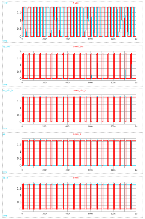
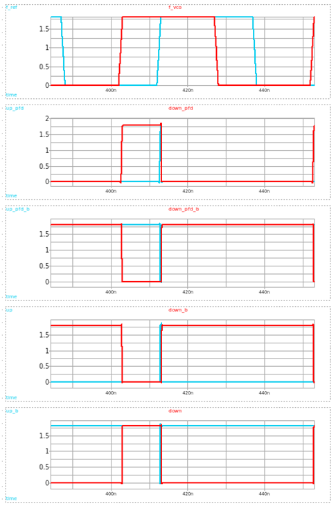
Figure 10. Input Pulse signals of the Second Condition
Fig.11 is similar to the aspects of fig.9.
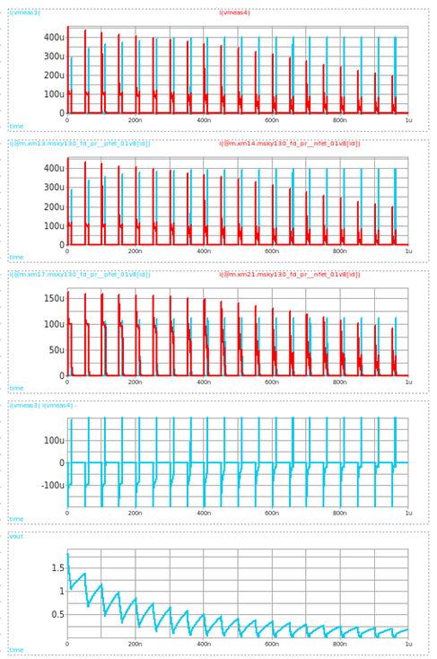
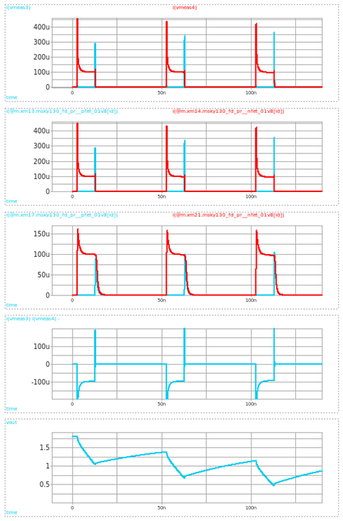
Figure 11. Current Flow in the Second Condition
3rd condition (F_REF same as F_VCO)
Similar to the 1st and 2nd condition, fig.12 is the pulse response of this transient response. The plots on the left show the full picture, and the plots on the right show the close-up pulses.
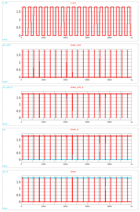
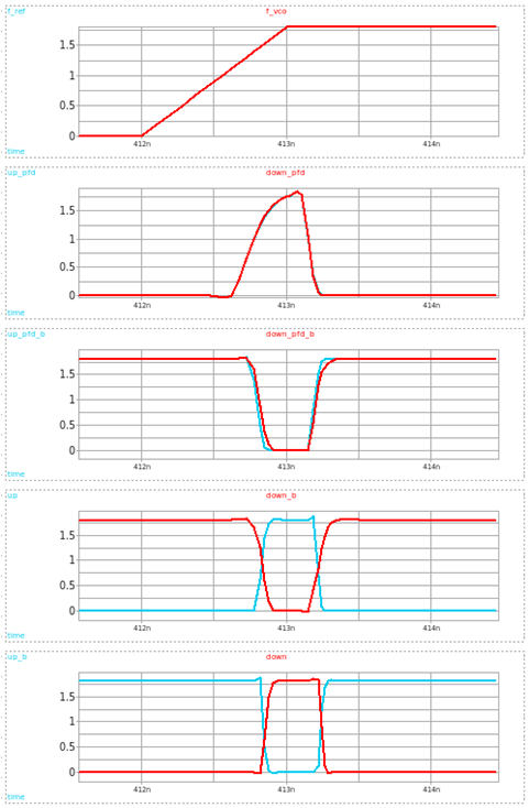
Figure 12. Input Pulse signals of the Third Condition
The 5th row of fig.13 shows the V_out result when the PLL is assumed to be in the lock state. To resolve its decreasing behavior, we can increase the length of M13 from 2um to 2.7um. The results are shown in fig.14
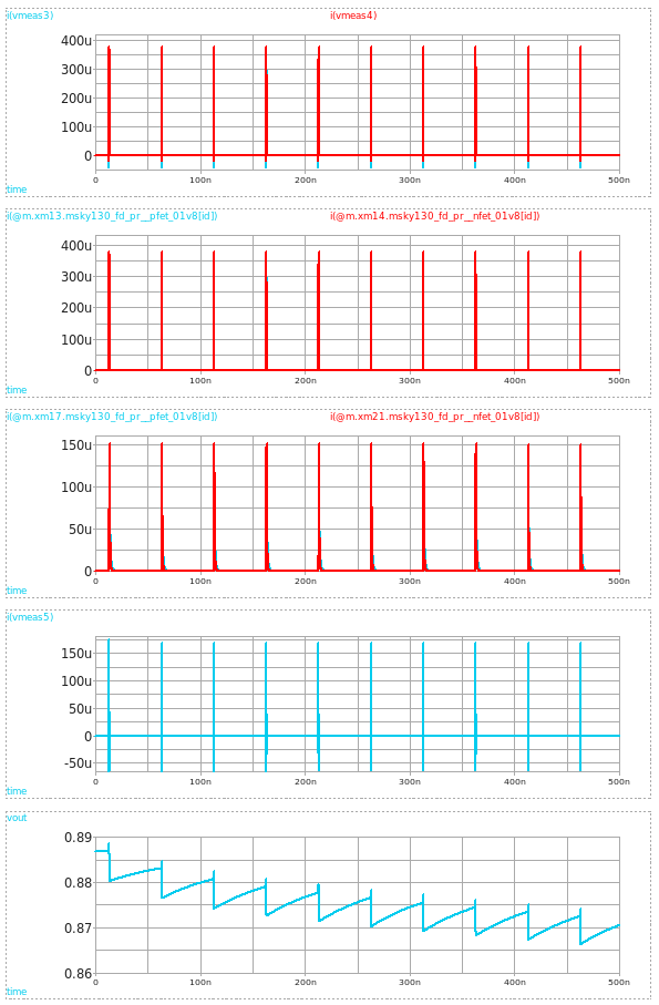
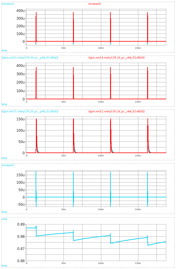
Figure 13. Current Flow in the Third Condition
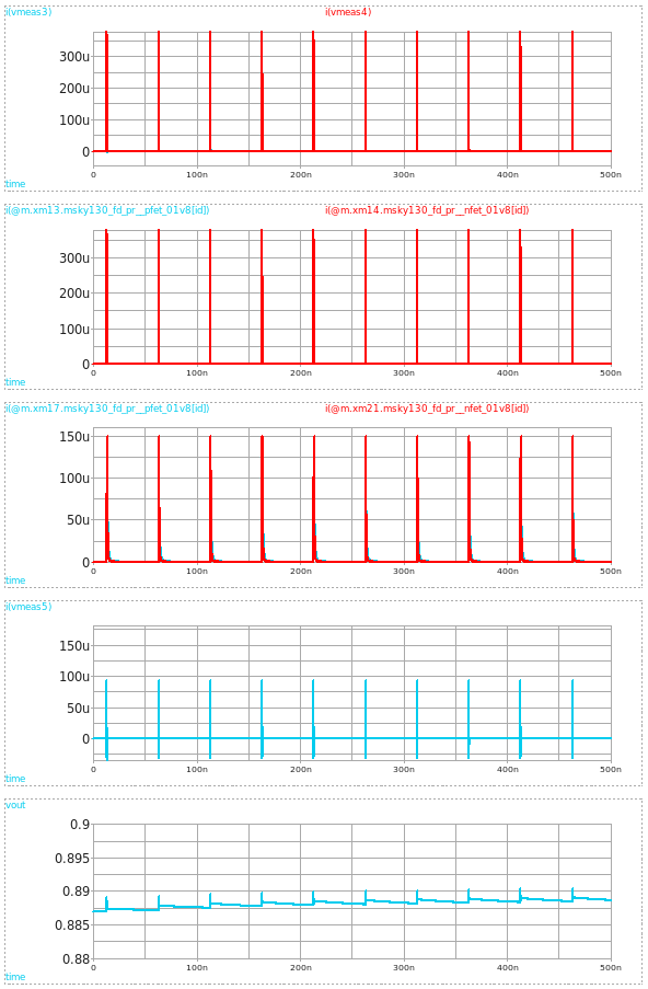
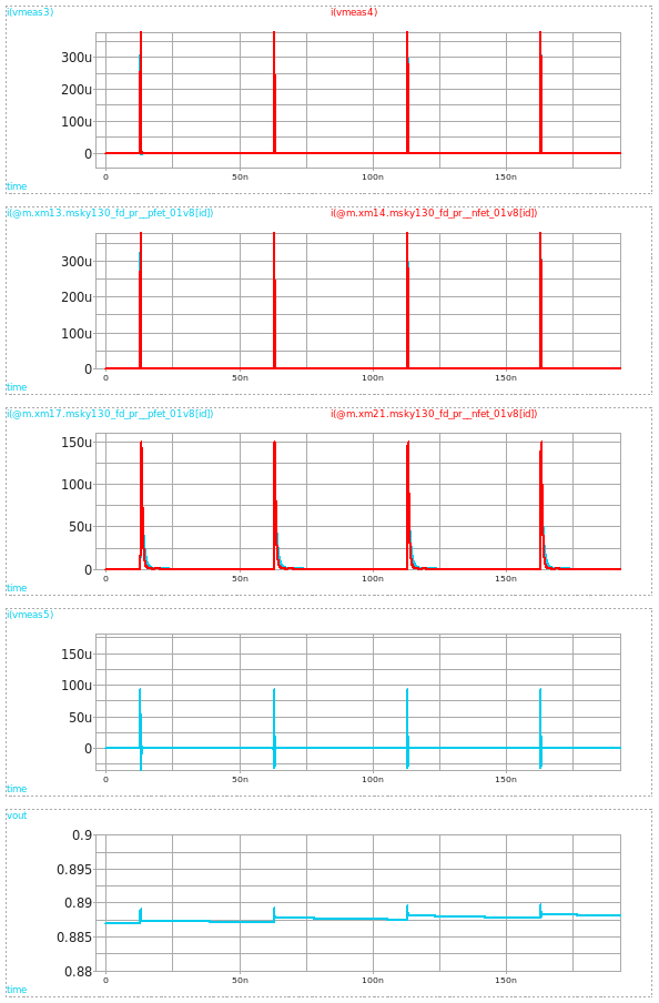
Figure 14. Current Flow in the Third Condition with Revised Transistor Sizes
4. Design Issues
This CP designs however, consists of the following issues.
4.1. Large Transistors
One of the problems in this design is that it requires large transistors for the reference current branches to mitigate channel length modulation. It reaches up to 200um X 1.5um in the largest transistors, which may take up lots of area in the chip die. Additionally, these large sizes naturally entail large parasitic capacitances leading to more problems when interacting with other PLL components with small capacitances. For example, when this CP is connected to the PFD from our previous design, the large capacitance introduces poor slew rates in the pulse interpretation. This property is the root problem that leads to the second issue.
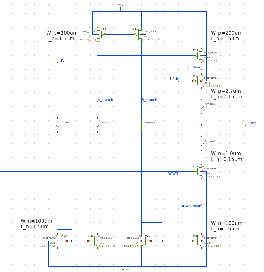
Figure 15. Big Transistors
4.2. Non-Linear Charge Pump
Fig.16 is a close-up picture of fig.13, it shows when the CP is locked in the lock state. It fails to provide 100uA from both PMOS and NMOS in the CP branch. This may not seem like an issue at the first glance because these two factors cancel each other out, thus not presenting any serious problems.
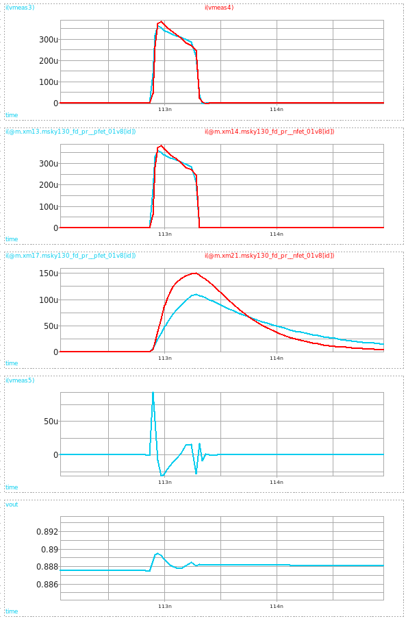
Figure 16. Excessive Current
However, this problem becomes clear when the F_REF and F_VCO delay offset is non-zero (e.g. +/-1ns, i.e. F_VCO delay =13ns).
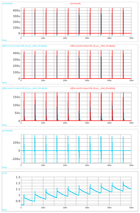
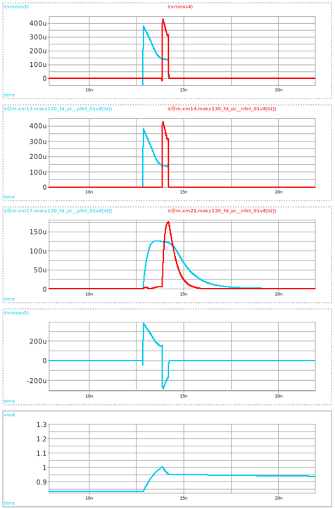
Figure 17. Excessive Current in Non-Zero Delay Offset Situations
As depicted in the 4th row of fig.17, it is difficult to say if the charge pump sources 100uA. Thus, we cannot dismiss the feasibility that this CP will have a non-linear functionality.
Charge Pump Dead Zone
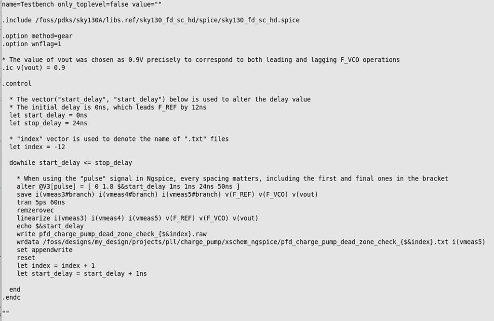
Figure 18. Delay Parameter Sweep SPICE code for CP Dead-Zone Validation
To check this CP function linearity, we write a new testbench for checking the CP dead zone. With this simulation, we can utilize its output “.txt” files to create a “Average charge pump current” VS “Delay Time” plot in Python. Not only does this check whether the design carries a CP dead zone but also confirms the linearity of the CP. SPICE code is given as fig.18, which will execute a parameter sweep of F_VCO delay time from 0ns ~ 24ns with 1ns timestep. The initial “Vout” node voltage is set to 0.9V accordingly to respond to both F_VCO operations in leading and lagging situations.
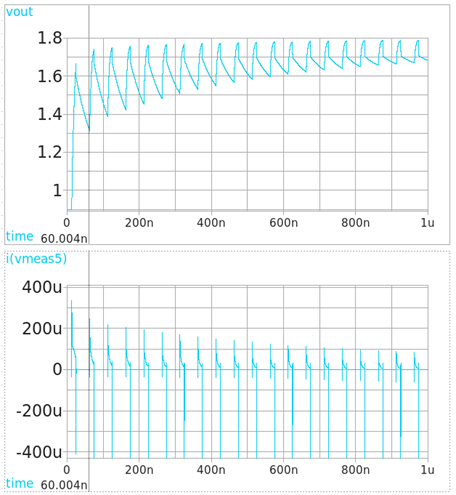
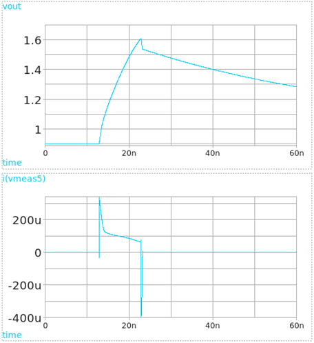
Figure.19 (Left: F_VCO is lagging by 10ns, 1us sim; Right: F_VCO is lagging by 10ns, 60ns sim)
One thing to note is that the transient signal runs for only 60ns, which feels too short for simulations. As the plot on the right in fig.19, when the simulation hits the first charge pump clock (approx. 0ns ~ 62.7ns), the v_out voltage already surges near the VDD. This leaves no margin for voltages in the succeeding clocks, so the following operations cannot exert the same voltage increase as they did in the first clock. Thus, they are forced to supply less than 100uA. So we capture only the action of the first clock to visualize the charge pump dead-zone behavior.
This is a matter in the voltage increment behavior of the loop filters. If we want to change this, we need to choose different loop filter parameters, as those are what create these actions. However, altering the loop filter parameter would mean that we also need alternative VCO configurations. Such measure is unnecessary because we have already configured our VCO through rigorous attempts.
After the simulation completes, we run "convert_txt_csv.py" which was introduced in the VCO design post, then we can check the CP dead zone by running a new code "current_per_delay_time.py"
The code for “current_per_delay_time.py” is shown below, and fig.20 is the result.
import pandas as pd
import numpy as np
import matplotlib.pyplot as plt
import os
import matplotlib.ticker as ticker

# File paths
intervals = np.arange(-12, 13, 1)  # Delay time intervals
file_paths = [f'pfd_charge_pump_dead_zone_check_2_{i}.csv' for i in intervals]

# Extract delay times from file names
delay_times = [float(os.path.basename(path).split('_')[-1].split('.')[0]) for path in file_paths]

# Function to integrate current over time up to 50ns
def integrate_current_upto_50ns(file_path):
    data = pd.read_csv(file_path, header=None)  # Load the CSV file
    time = data[0]  # Time is in the first column
    current = data[1]  # Current is in the second column

    # Filter data to include only time values <= 50 ns (50e-9 seconds)
    filtered_data = data[time <= 50e-9]
    time_filtered = filtered_data[0]
    current_filtered = filtered_data[1]

    # Integrate current over time to get charge
    charge = np.trapz(current_filtered, x=time_filtered)  # Use time as x-axis for integration
    avg_current = charge / (time_filtered.iloc[-1] - time_filtered.iloc[0])  # Average current over time
    return avg_current

# Calculate average currents for all files
average_currents = [integrate_current_upto_50ns(file_path) for file_path in file_paths]

# Plotting "Charge Pump Current vs Delay Time" for data up to 50ns
plt.figure(figsize=(10, 6))
plt.plot(delay_times, average_currents, marker='o', linestyle='-', color='b')

# Add annotations for average current values
for x, y in zip(delay_times, average_currents):
    plt.text(x, y, f'{y:.2e}', fontsize=9, ha='right', va='bottom')

plt.xlabel("Delay Time (ns)")
plt.ylabel("Average Charge Pump Current (A) (up to 50 ns)")
plt.title("Charge Pump Current vs Delay Time (Up to 50 ns)")

# Set grid and ticks to show 1 ns intervals
plt.grid(True, which='both', linestyle='--', linewidth=0.5)
plt.xticks(np.arange(-12, 13, 1))  # Setting x-axis ticks at every 1 ns interval
plt.gca().xaxis.set_major_locator(ticker.MultipleLocator(1))
plt.gca().yaxis.set_major_locator(ticker.MaxNLocator(integer=True))

# Save the plot before showing it
plt.savefig('charge_pump_current_vs_delay_time_upto_50ns.png')

# Now show the plot
plt.show()
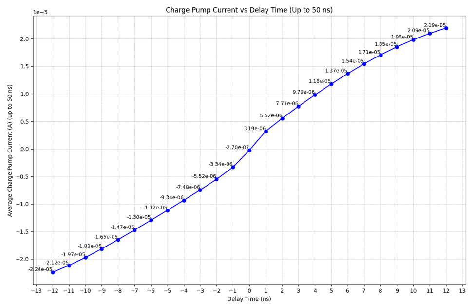
Figure 20. Current VS. Delay Plot
This issue arises from the PMOS and NMOS current sourcing branches not sourcing the proper 100uA.
One might think of a solution by changing the length of M13 (0.15um to 0.5um) and M14 (0.15um to 1.0um), to match the 100uA output, which is shown in fig.21.
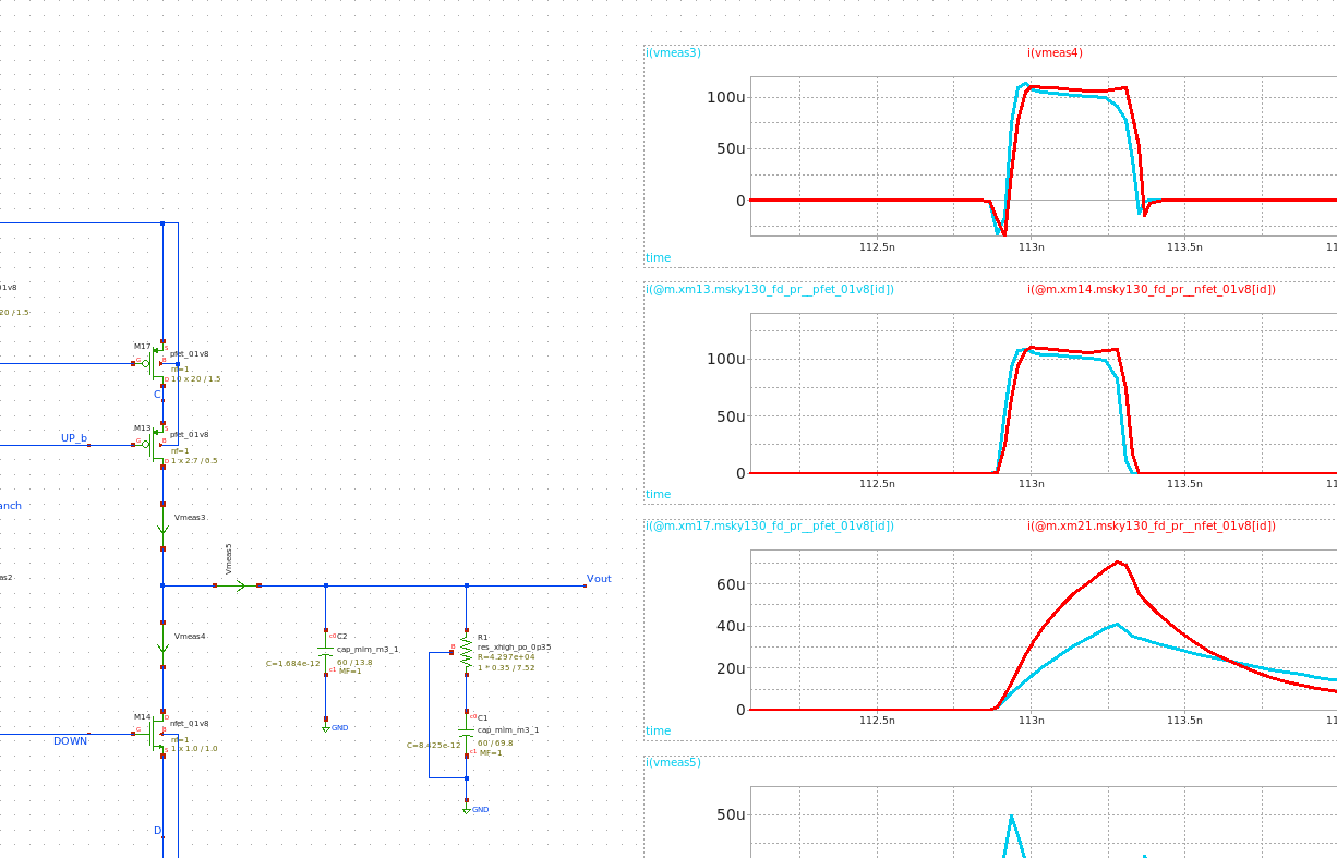
Figure 21. Revised Charge Pump Transistor Sizes
However, this contradicts DC analysis as shown in fig.22. It shows severe current mismatches between the PMOS and NMOS current branch in the operating voltage range.
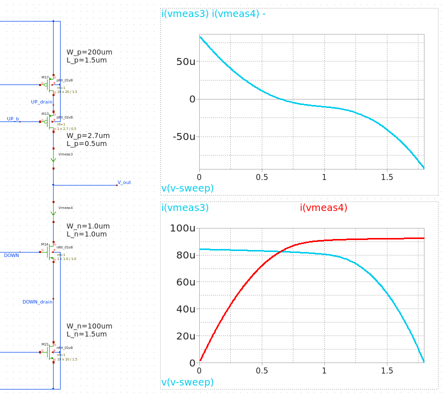
Figure 22 DC Mismatch
The result proves that this CP design carries two major issues.
First, this CP topology has immensely large transistors, especially for the current mirroring branches. Second, the CP operation is significantly non-linear. While there could be possible solutions, the natural trait of the big transistors being plagued with big parasitic capacitances limits the number of options.
In the next post, a new topology will be suggested in nanoscale design to resolve the above two issues.
Discussion
Comments
Share questions, corrections, or notes through GitHub.